Kelton and Krugman on IS-LM and MMT
The MMT debates continue apace. New critiques — the good, the bad and the ugly — appear daily. Amidst the chaos, a guest post on Alphaville from three MMT authors stood out: the piece responded directly to various criticisms while discussing the policy challenges associated with controlling demand and inflation when fiscal policy is the primary macro stabilisation tool. These are the debates we should be having.
Unfortunately, it is one step forward, two steps backwards: elsewhere Stephanie Kelton and Paul Krugman have been debating across the pages of the Bloomberg and the New York Times websites. The debate is, to put it politely, a mess.
Krugman opened proceedings with a critique of Abba Lerner’s Functional Finance: the doctrine that fiscal policy should be judged by its macroeconomic outcomes, not on whether the financing is “sound”. Lerner argued that fiscal policy should be set at a position consistent with full employment, while interest rates should be set at a rate that ensures “the most desirable level of investment”. Krugman correctly notes the lack of precision in Lerner’s statement on interest rates. He then argues that, “Lerner neglected the tradeoff between monetary and fiscal policy”, and that if the rate of interest on government debt exceeds the rate of growth, either the debt to GDP ratio spirals out of control or the government is forced to tighten fiscal policy.
Kelton hit back, arguing that Krugman’s concerns are misplaced because interest rates are a policy variable: the central bank can set them at whatever level it likes. Kelton points out that Krugman is assuming a “crowding out” effect: higher deficits lead to higher interest rates. Kelton argues that instead of “crowding out”, Lerner was concerned about “crowding in”: the “danger” that government deficits would push down the rate of interest, stimulating too much investment. Putting aside whether this is an accurate description of Lerner’s view, MMT does diverge from Lerner on this issue: since MMT rejects a clear link between interest rates and investment, the MMT proposal is simply to set interest rates at a low level, or even zero, and leave them there.
So far, this looks like a straightforward disagreement about the relationship between government deficits and interest rates: Krugman says deficits cause higher interest rates, Kelton says they cause lower interest rates (although she also says interest rates are a policy variable — this apparent tension in Kelton’s position is resolved later on)
Krugman responded. This is where the debate starts to get messy. Krugman takes issue with the claim that the deficit should be set at the level consistent with full employment. He argues that at different rates of interest there will be different levels of private sector spending, implying that the fiscal position consistent with full employment varies with the rate of interest. As a result, the rate of interest isn’t a pure policy variable: there is a tradeoff between monetary and fiscal policy: with a larger deficit, interest rates must be higher, “crowding out” private investment spending.
Krugman’s argument involves two assumptions: 1) there exists a direct causal relationship between the rate of interest and the level of private investment expenditure, and, 2) the central bank will react to employment above “full employment” with higher interest rates. He illustrates this using an IS curve and a vertical “full employment” line (see below). He declares that “this all seems clear to me, and hard to argue with”.
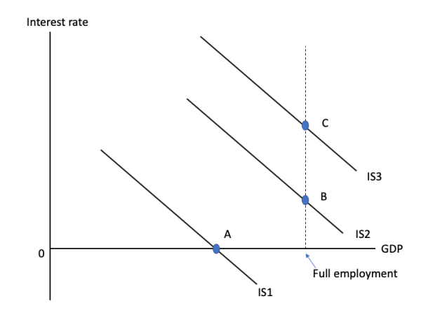
Interest
rate
|
| |
| \ |
| \ |
| \ |
| \|
| \C
| \C
| \ |\
| \ | \IS3
| \|
| \B
| \ | \IS3
| \|
| \B
| \ |\
| \ | \IS2
| \A |
|_________\____|______ GDP
0| \ ↑Full
| \ employment
| IS1
|
| \ | \IS2
| \A |
|_________\____|______ GDP
0| \ ↑Full
| \ employment
| IS1
|
At this point the debate still appears to remain focused on the core question: do government deficits raise or lower the rate of interest? By now, Krugman is baffled with Kelton’s responses:
It seems as if she’s saying that deficits necessarily lead to an increase in the monetary base, that expansionary fiscal policy is automatically expansionary monetary policy. But that is so obviously untrue – think of the loose fiscal/tight money combination in the 1980s – that I hope she means something different. Yet I can’t figure out what that different thing might be.
This highlights two issues: first, how little of MMT Krugman has bothered to absorb, and, second, how little MMTers appear to care about engaging others in a clear debate. Kelton, following the MMT line, is tacitly assuming that all deficits are monetised and that issuing bonds is an additional, and possibly unnecessary, “sterilisation” operation. Under these assumptions, deficits will automatically lead to an increase in central bank reserves and therefore to a fall in the money market rate of interest. But Kelton at no point makes these assumptions explicit. To most people, a government deficit implicitly means bond issuance, in correspondence with the historical facts.
So Krugman and Kelton have two differences in assumptions that matter here. First, Krugman assumes a mechanical relationship between interest rates and investment and thus a downward sloping IS curve, while Kelton rejects this relationship. Second, they are assuming different central bank behaviour. Krugman assumes that the central bank will react to fiscal expansion with tighter monetary policy in the form of higher interest rates: the central bank won’t allow employment to exceed the “full employment” level. Kelton assumes, firstly, that fiscal policy can be set at the “full employment” level, without any direct implications for interest rates and, secondly, that deficits are monetised so that money market rates fall as the deficit expands.
The “debate” heads downhill from here. Krugman asks several direct questions, including “[does] expansionary fiscal policy actually reduce interest rates?”. Kelton responds, “Answer: Yes. Pumping money into the economy increases bank reserves and reduces banks’ bids for federal funds. Any banker will tell you this.” Even now, neither party seems to have identified the difference in assumptions about central bank behaviour.
The debate then shifts to IS-LM. Krugman asks if Kelton accepts the overall framework of discussion — the one he previously noted “all seems clear to me, and hard to argue with”. Kelton responds that, no, MMT rejects IS-LM because it is “not stock-flow consistent”, while also correctly noting that Krugman simply assumes that investment is a mechanical function of the rate of interest.
In fact, Krugman isn’t even using an IS-LM model — he has no LM curve — so the “not stock flow consistent” response is off target. The stock-flow issue in IS-LM derives from the fact that the model solves for an equilibrium between equations for the stock of money (LM), and investment and saving (IS) which are flow variables. But without the LM curve it is a pure flow model: Krugman is assuming, as does Kelton, that the central bank sets the rate of interest directly. So Kelton’s claim that “his model assumes a fixed money supply, which paves the way for the crowding-out effect!” is incorrect.
Similarly, Kelton’s earlier statement that Krugman “subscribes to the idea that monetary policy should target an invisible ‘neutral rate'” makes little sense in the context of Krugman’s IS model: there is no “invisible” r* in a simple IS model of the type Krugman is using: the full employment rate of interest can be read straight off the diagram for any given fiscal position.
Krugman then took to Twitter, calling Kelton’s response “a mess”, while still apparently failing to spot that they are talking at cross purposes. Kelton hit back again arguing that,
The crude, IS-LM interpretation of Keynes demonstrates that, under normal conditions, an increase in deficit spending will push up interest rates and lead to some crowding-out of investment spending. There is no room for a technical analysis of monetary operations in that framework.
Can this discussion be rescued? Can MMT and IS-LM be reconciled? The answer, I think, turns out to be, “yes, sort of”.
I wasn’t the only person pondering this question: several people on Twitter went back to this post by Nick Rowe where he tries to “reverse engineer” MMT using the IS-LM model, and comes up with the following diagram:
Report this ad
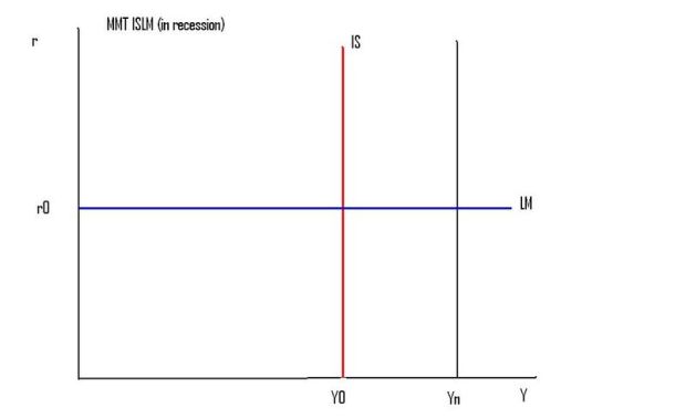 Does this help? I think it does. In fact, this is exactly the diagram used by Victoria Chick in 1973, in The Theory of Monetary Policy, to describe what she calls the “extreme Keynesian model” (bottom right):
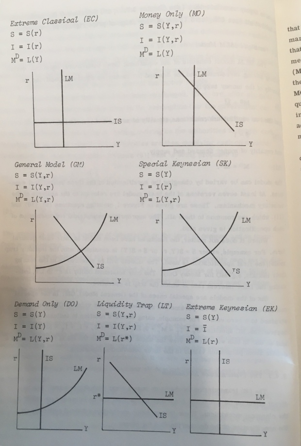
Report this ad
So how do we use this diagram to resolve the Krugman-Kelton debate? Before answering, it should be noted that MMTers are correct to point out problems with the IS-LM framework. Some are listed in this article by Mario Seccareccia and Marc Lavoie who conclude that IS-LM should be rejected, but “if one were to hold one’s nose,” the “least worst” configuration is what Chick calls the “extreme Keynesian” version.
To see how we resolve the debate, and at the risk of repeating myself, recall that Krugman and Kelton are talking about two different central bank reactions. In Krugman’s IS model, the central bank reacts to looser fiscal policy with higher interest rates. Kelton, on the other hand, is talking about how deficit monetisation lowers the overnight money market rate. Kelton’s claim that a government deficit reduces “interest rates” is largely meaningless: it is just a truism. Flooding the overnight markets with liquidity will quickly push the rate of interest to zero, or whatever rate of interest the central bank pays on reserve balances. It is a central bank policy choice: the opposite of the one assumed by Krugman.
But what effect will this have on the interest rates which really matter for investment and debt sustainability: the rates on corporate and government debt? The answer is “it depends” — there are far too many factors involved to posit a direct mechanical relationship.
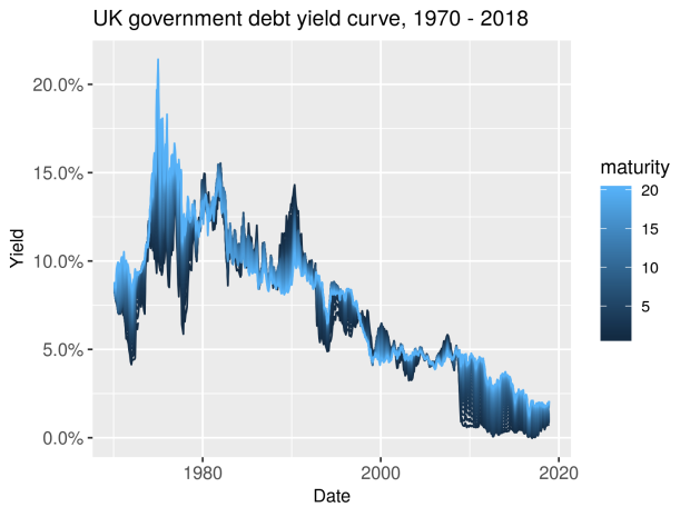
This brings a problem that is lurking in the background into sight. Both Kelton and Krugman are talking about “interest rates” or “the interest rate” as if there were a single rate of interest, or that all rates move together — the yield curve shifts bodily with movements of the policy rate. As the chart below shows, even for government debt alone this is a problematic assumption.
Now, in the original IS-LM model, the LM curve is supposed to show how changes in the government controlled “money supply” affects the long term bond rate of interest. This is because, for Keynes, the rate of interest is the price of liquidity: by giving up liquidity (money) in favour of bonds, investors are rewarded with interest payments. But the problem with this is that we know that central banks don’t set the “money supply”: they set a rate of interest. So, it has become customary to draw a horizontal MP curve, allegedly representing an elastic supply of money at the rate of interest set by the central bank. But note that in switching from a sloping to a horizontal LM curve, the “interest rate” has switched from the long bond rate to the rate set by the central bank.
So how is the long bond rate determined in the horizontal MP model? The answer is it isn’t. As in the more contemporary three-equation IS-AS-MP formulation, it is just assumed that the central bank fixes the rate of interest that determines total spending. In switching from the upward sloping LM curve to a horizontal MP curve, the crude approximation to the yield curve in the older model is eliminated.
What of the IS curve? Kelton is right that a mechanical relationship between interest rates and investment (and saving) behaviour is highly dubious. If we assume that demand is completely interest-inelastic, then we arrive at the “extreme Keynesian” vertical IS curve. But does Kelton really think that sharp Fed rate hikes will have no effect on total spending? I doubt it. As Seccareccia and Lavoie note, once the effects of interest rates on the housing market are included, a sloping-but-steep IS curve seems plausible.
Report this ad
Now, does the “extreme Keynesian” IS-LM model, all the heroic assumptions notwithstanding, represent the MMT assumptions? I think, very crudely, it does. The government can set fiscal policy wherever it likes, both irrespective of interest rates and without affecting interest rates: the IS curve can be placed anywhere along the horizontal axis. Likewise, the central bank can set interest rates to anything it likes, again without having any effect on total expenditure. This seems a reasonable, if highly simplified approximation to the standard MMT assumptions that fiscal policy and monetary policy can be set entirely independently of each other.
But is it useful? Not really, other than perhaps in showing the limitations of IS-LM. The only real takeaway is that we deserve a better quality of economic debate. People with the visibility and status of Kelton and Krugman should be able to identify the assumptions driving their opponent’s conclusions and hold a meaningful debate about whether these assumptions hold — without requiring some blogger to pick up the pieces.
IS-LMとMMTに関するKeltonとKrugman
Jo Michell 3月6、2019
MMTの議論は急速に進んでいます。新しい批評 - 善、悪、醜い - が日々現れています。混乱の中で、MMTの3人の作者によるAlphavilleのゲスト投稿が際立っていました。財政政策が主要なマクロ安定化ツールであるとき、需要とインフレを制御することに関連する政策課題を議論しながら作品はさまざまな批判に直接答えました。これらは私達が持っているべきである議論です。
残念なことに、それは一歩前進、二歩後退です。他の場所では、Stephanie Kelton氏とPaul Krugman氏が、ブルームバーグとニューヨークタイムズのWebサイトのページで議論しています。議論は、それを丁寧に言うと、混乱です。
Krugmanは、Abba Lernerの機能金融に対する批判を受けて訴訟を開始した。財政政策は資金調達が「健全」であるかどうかではなく、そのマクロ経済的成果によって判断されるべきであるという教義。ラーナー氏は、財政政策は完全雇用と一致する位置に設定すべきであり、金利は「最も望ましい水準の投資」を保証する速度に設定すべきであると主張した。 Krugmanは、Lernerの金利に関する声明の正確さの欠如を正しく指摘しています。そして彼は、「ラーナーは金融政策と財政政策の間のトレードオフを無視していた」、そして政府の債務に対する利子率が成長率を超えると、債務対GDP比が暴走するか、政府が締め付けを余儀なくすると主張する。財政政策。
Kelton氏は、金利は政策変数であるため、Krugmanの懸念は見当違いであると主張し、中央銀行はそれを好きなレベルに設定することができる。 Kelton氏は、Krugmanが「圧倒的な」影響を想定していると指摘しています。赤字が増加すると金利が上昇することになります。ケルトン氏は、「混雑」ではなく、「混雑」について懸念していたと語った。政府の赤字が金利を押し下げて投資を刺激しすぎるという「危険」。これがLernerの見解の正確な説明であるかどうかを脇に置いて、MMTはこの問題についてLernerから分岐します:MMTは金利と投資の明確な関連性を拒絶するので、MMT提案は単に金利を低水準、あるいはゼロに設定することですそしてそれらをそこに残しなさい。
これまでのところ、これは政府の赤字と金利の関係についての直接的な意見の不一致のように見えます:Krugmanは赤字がより高い金利を引き起こすと言います、Keltonは彼らがより低い金利を引き起こすと言いますケルトンの立場は後で解決される)
クルーグマンは答えた。これは議論が乱雑になり始めるところです。 Krugmanは、赤字は完全雇用と一致する水準に設定されるべきであるという主張に問題を投げかけている。同氏は、利子率が異なると民間部門の支出水準も異なることを示唆しており、これは、完全雇用と一致する財政状態は利子率によって異なることを意味している。その結果、金利は純粋な政策変数ではありません。金融政策と財政政策の間にはトレードオフがあります。赤字が大きくなればなるほど、金利はより高くなるはずです。
Krugmanの主張は、1)利子率と民間投資支出の水準との間に直接的な因果関係があり、2)中央銀行がより高い金利で「完全雇用」以上の雇用に反応するという2つの仮定を含んでいる。彼はこれをIS曲線と垂直の「完全雇用」線を使って説明している(下記参照)。彼は、「これはすべて私には明白であり、議論するのは難しいようだ」と宣言する。
この広告を報告
現時点では、議論は依然として中心的な問題、すなわち政府の赤字が金利を引き上げるか引き下げるかに集中しているように思われる。現在までに、KrugmanはKeltonの返答に困惑している。
赤字が必然的に貨幣基盤の増加につながると言っているように、拡大的な財政政策は自動的に拡大的な金融政策であると彼女は言っているようです。しかし、それは明らかに不正確です - 1980年代の緩い財政とタイトマネーの組み合わせについて考えてください - 彼女が何か違うことを意味することを私は願っています。それでも、その別のことが何なのかわからない。
これは2つの問題に焦点を当てています。1つは、MMT Krugmanが吸収することに煩わされていないこと、もう1つは、明確な議論に他のMMTを参加させることに関心がないことです。ケルトンは、MMTの方針に従って、すべての赤字が金銭化され、債券の発行は追加の、そしておそらく不要な「滅菌」作戦であると暗黙のうちに仮定している。これらの仮定の下では、赤字は自動的に中央銀行の準備金の増加につながり、したがって、短期金融市場金利の低下につながります。しかし、ケルトンはこれらの仮定を明確にしていません。ほとんどの人にとって、政府の赤字は歴史的事実と一致して、暗黙のうちに債券発行を意味します。
したがって、KrugmanとKeltonには、ここで重要な2つの違いがあります。第一に、Krugmanは金利と投資との間の機械的な関係、したがって下降勾配のIS曲線を仮定しますが、Keltonはこの関係を拒否します。第二に、彼らは異なる中央銀行の行動を想定しています。 Krugmanは、中央銀行がより高い金利という形でより厳格な金融政策を用いて財政拡大に反応すると仮定している。中央銀行は雇用が「フル雇用」レベルを超えることを認めていない。ケルトン氏は、第一に、金利に直接影響を与えることなく、財政政策を「完全雇用」レベルに設定することができ、第二に、赤字が拡大するにつれてマネーマーケットレートが下がるように赤字を金銭化すると仮定する。
「議論」はここから下り坂に向かう。 Krugmanはいくつかの直接的な質問をします。「拡大財政政策は実際に金利を引き下げますか」など。ケルトンはこう答えます。経済にお金を注ぎ込むことは、銀行の準備金を増やし、連邦資金に対する銀行の入札を減らします。今でも、どちらの当事者も中央銀行の行動に関する仮定の違いを識別していないようです。
その後、議論はIS-LMに移ります。 Krugmanは、Keltonが全体的な議論の枠組みを受け入れたかどうかを尋ねた - 彼が以前に「すべては私には明白であり、議論するのは難しいように思われる」と述べたもの。 Kelton氏は、Krugmanは単に投資は利子率の機械的関数であると仮定しているだけでなく、「MMFはIS-LMを「在庫フローの一貫性がない」ので拒否している」と答えた。
実際、Krugmanは、IS-LMモデルを使用しているわけでもありません - LM曲線がないため、「在庫フローが一貫していない」という回答は目標外です。 IS-LMのストックフローの問題は、モデルが貨幣の在庫の方程式(LM)と投資と貯蓄(IS)との間の平衡をフロー変数であることから解くという事実から派生します。しかしLM曲線がなければ、それは純粋な流動モデルです:Krugmanは、Keltonがそうであるように、中央銀行が直接金利を設定すると仮定しています。ケルトンの主張は、「彼のモデルは固定のマネーサプライを前提としているため、クラウドアウト効果に道を開くことができます」というのは正しくありません。
同様に、Krugmanが「金融政策は目に見えない「中立的利率」を目標とすべきであるという考えに同意している」というKeltonの以前の声明は、KrugmanのISモデルの文脈ではほとんど意味がありません。 Krugmanが使用しているタイプ:任意の特定の財政ポジションについて、全雇用金利をダイアグラムから直接読み取ることができます。
KrugmanはそれからTwitterに連れて行き、Keltonの返事を「めちゃくちゃ」と呼んだ。ケルトンはまた次のように主張した。
ケインズの粗野なIS-LMの解釈は、通常の状況下では、赤字支出の増加が金利を押し上げ、投資支出のいくらかの混雑を招くことを示している。その枠組みの中で金融業務の技術的な分析の余地はありません。
この議論は救助できますか? MMTとIS-LMは調整できますか?その答えは、「はい、そのとおり」です。
私はこの質問を熟考している唯一の人ではありませんでした。Twitterの何人かの人々がNick Roweによってこの投稿に戻り、そこで彼はIS-LMモデルを使ってMMTを「リバースエンジニアリング」しようとします。
Does this help? I think it does. In fact, this is exactly the diagram used by Victoria Chick in 1973, in The Theory of Monetary Policy, to describe what she calls the “extreme Keynesian model” (bottom right):
これは助けになりますか? そうだと思います。 実際、これはまさに1973年にビクトリア・チックが「極端なケインジアン・モデル」(右下)と呼んでいるものを記述するために金融政策の理論で使用した図です。
では、どのようにしてこの図を使ってKrugman-Keltonの議論を解決するのでしょうか。答える前に、MMTersはIS-LMフレームワークの問題を指摘するのが正しいということに注意すべきです。この記事ではIS-LMを却下すべきだと結論づけているMario SeccarecciaとMarc Lavoieがリストしていますが、「最悪の」設定は「極端なケインジアン」バージョンと呼ばれるものです。
私たちがどのように議論を解決し、そして私自身を繰り返す危険性があるかを見るために、KrugmanとKeltonは2つの異なる中央銀行の反応について話していることを思い出してください。 KrugmanのISモデルでは、中央銀行はより高い金利でより緩やかな財政政策に反応します。一方、ケルトン氏は、赤字の貨幣化が一晩のマネーマーケットレートをどのように低下させるかについて話している。政府の赤字が「金利」を引き下げるというケルトンの主張は、ほとんど意味がない。それは単なる真実である。翌日物市場に流動性をあふれさせることは、利子率を速やかにゼロに、あるいは中央銀行が準備金残高に対して支払う利子率を急上昇させるでしょう。それは中央銀行の政策選択です:Krugmanによって仮定されたものの反対です。
しかし、これが投資と債務の持続可能性にとって本当に重要な金利、企業債務と政府債務の金利にどのような影響を与えるでしょうか。答えは「それが依存する」です - 直接的な機械的関係を確立するためには、あまりにも多くの要因が関係しています。
これは、背景に潜んでいる問題を目の当たりにします。 KeltonとKrugmanはどちらも、「金利」または「金利」について、単一の金利があるかのように、またはすべての金利が連動しているように話しています。イールドカーブは、政策金利の変動に伴い変化します。下のグラフが示すように、政府債務だけでもこれは問題のある前提です。
さて、元のIS-LMモデルでは、LM曲線は政府が管理する「マネーサプライ」の変化が長期債券利子率にどのように影響するかを示すと考えられています。これは、ケインズにとって利子率は流動性の価格であるためである。債券を支持して流動性(お金)を放棄することによって、投資家は利子の支払いで報われる。しかし、これに関する問題は、中央銀行が「マネーサプライ」を設定しないことを私たちが知っているということです。彼らは利子率を設定します。そのため、中央銀行が設定した利子率で弾力的な貨幣供給を表すとされる水平MP曲線を描くことが慣例となっている。しかし、スロープから水平LMカーブへの転換では、「金利」がロングボンド金利から中央銀行が設定した金利に切り替わったことに注意してください。
それでは、水平MPモデルでロングボンドレートはどのように決定されるのでしょうか。答えはそうではありません。より現代的な3式のIS-AS-MPの定式化のように、中央銀行が総支出を決定する金利を決定すると仮定されているだけです。上向きのLM曲線から水平方向のMP曲線への切り替えでは、古いモデルのイールドカーブへの大まかな近似は削除されます。
IS曲線は何ですか?ケルトンは、金利と投資(そして貯蓄)行動との間の機械的関係が非常に疑わしいと考えています。需要が完全に金利非弾力的であると仮定すると、「極端なケインジアン」の垂直IS曲線にたどり着きます。しかし、ケルトンは実際には急激なFRBの利上げは総支出に影響を及ぼさないであろうと考えていますか?疑わしい。 SeccarecciaとLavoieが述べているように、住宅市場に対する金利の影響が含まれると、傾斜が急なIS曲線がもっともらしいと思われる。
この広告を報告
さて、「極端なケインジアン」のIS-LMモデルは、それにもかかわらずすべての英雄的な仮定であり、MMTの仮定を表しているのでしょうか。非常におおまかに言って、そうだと思います。政府は、金利に関係なく、また金利に影響を与えることなく、財政政策を好きなところに設定できます。IS曲線は、横軸のどこにでも配置できます。同様に、中央銀行は、総支出に影響を与えることなく、利子率を好きな値に設定することができます。財政政策と金融政策は互いに完全に独立して設定できるという標準的なMMTの仮定に非常に単純化された近似であれば、これは合理的に思えます。
しかし、それは便利ですか? IS-LMの限界を示すこと以外に、実際にはそうではありません。唯一の本当のテイクアウトは、我々がより質の高い経済的議論に値するということです。 KeltonとKrugmanの可視性と地位を持つ人々は、相手の結論を導いた仮定を特定し、これらの仮定が成り立つかどうかについて有意義な議論をすることができます。
参考:
ミッチェル2019#28後半458~に対応
貨幣供給が内生的に決定されているという事実は、LMが政策金利に対して水平になることを意味する。したがって、金利の変動はすべて中央銀行によって設定され、資金はその金利で弾力的に需要に応じて供給されます。この場合、IS曲線の変化は金利に影響を与えません。
政策的見地から、これは中央銀行がマネーサプライを増やすことによって失業を解決することができるという単純な概念に欠陥があることを意味します。
IS-LM Framework – Part 6
I am now using Friday’s blog space to provide draft versions of the Modern Monetary Theory textbook that I am writing with my colleague and friend Randy Wray. We expect to complete the text during 2013 (to be ready in draft form for second semester teaching). Comments are always welcome. Remember this is a textbook aimed at undergraduate students and so the writing will be different from my usual blog free-for-all. Note also that the text I post is just the work I am doing by way of the first draft so the material posted will not represent the complete text. Further it will change once the two of us have edited it.
Previous Parts to this Chapter:
Previous Parts to this Chapter:
- The IS-LM Framework – Part 1
- The IS-LM Framework – Part 2
- The IS-LM Framework – Part 3
- The IS-LM Framework – Part 4
- The IS-LM Framework – Part 5
Chapter 16 – The IS-LM Framework
[PREVIOUS MATERIAL HERE IN PARTS 1 to 5]
16.6 Introducing the price level – the Keynes and Pigou effects
[CONTINUING FROM LAST WEEK – WITH REVISED DIAGRAM AND PIGOU EFFECT ADDED]
Figure 16.10 depicts a family of LM curves with each individual curve corresponding to a different price levels (P0 is the highest price and P3 is the lowest price).
The introduction of the price level now means that the interest rate-income equilibrium is now contingent on the price level. If there is a different price level, the equilibrium changes as noted.
This means that within this framework, the national income equilibrium can shift without any change in monetary or fiscal policy settings if the price level changes.
Figure 16.10 The Keynes Effect


This observation was central to the debates between Keynes and the classical economists during the 1930s, which we examined in detail in Chapter 15.
Assume that the economy is currently at Point A, where the interest-rate is i0 and national income is Y0. The general price level is P0.
The full employment output level is at YFE, so that the current equilibrium corresponds to what Keynes would refer to as a underemployment equilibrium.
At Point A, the product and money markets are in equilibrium but there is an output gap and there would be mass unemployment in the labour market as a consequence.
Keynes considered this to be the general case for a monetary economy and depicted the neo-classical model as a special case in which the equilibrium that emerged was also consistent with full employment. For Keynes, a monetary economy could be in equilibrium at any level of national income.
The neo-classical response to this was that unless we impose fixed wages on the model, the persistent mass unemployment would eventually lead to falling nominal wages and prices.
While this might not lead to a fall in the real wage (if nominal wages and prices fall proportionately), which would negate the traditional neo-classical route to full employment via marginal productivity theory, the fact remains that the lower price level increases real balances in the economy.
The reasoning that follows is that the reduction in prices leads to a decline in the transactions demand for money at every level of income because goods and services are now cheaper.
With the nominal stock of money fixed, the expansion of real balances combined with a decline in the demand for liquidity, results in a decline in the rate of interest.
As long as future expectations of returns are not affected adversely by the deflationary environment, the reduction in the rate of interest, stimulates investment spending, which leads to increased aggregate output and income via the multiplier effect.
As long as there is an output gap, deflation will continue and the interest rate will continue to fall until the economy is at full employment.
The link between real balances and the interest rate was referred to as the Keynes effect.
In terms of Figure 16.10, the LM curve shifts outwards as the price level falls and the rising investment is depicted as a movement along the IS curve.
For example, if the price level fell to P1, the LM curve would shift and a new IS-LM equilibrium would result at Point B, with the interest rate at i1 and national income is Y1. Under the circumstances depicted this is not a full employment level of national income.
As a result of this observation, the neo-classical economists argued that an underemployment equilibrium was a special case when wages and prices were fixed given that flexible prices could reduce the output gap and unemployment via LM curve shifts.
The view that Keynes’ underemployment equilibrium was a special case of the more general flexible price model became known as the Neo-classical synthesis. This approach recognised that aggregate demand drove income and employment (the so-called Keynesian contribution) but that the economy would tend to full employment if wages and prices were flexible (the Classical contribution).
Note that the capacity of the Keynes effect to deliver output and employment gains is limited. If there is a liquidity trap (iLT) then the maximum expansion in national income that is possible via falling prices would be YL at Point C (where the IS curve intersects with the flat segment of the LM curve.
At that point, there would still be unemployment and if wages and prices were flexible and behaved according to the Classical labour market dynamics, the price level would continue to fall, say to P3.
The LM curve would continue to shift out but there would be no further expansion in national income beyond YL because the increase in real balances would not reduce the interest rate below iLT.
The classical route to full employment thus would require the full employment level of national income to lie at a point where the intersection of the IS-LM curves produced an equilibrium interest that that was equal to or above iLT.
The Keynes effect is so-named because the expansion that follows a reduction in the price level occurs through a rise in aggregate demand – first, through the interest=rate stimulus to investment, and, second, through the standard expenditure multiplier inducing higher consumption expenditure.
However, as we learned in Chapter 15, Keynes did not support wage and price cuts as a way to achieve full employment. He considered the social consequences of wage cuts to be unacceptable and instead advocated increasing the nominal money supply as the way to increase real balances.
But the limits to expansion posed by the possible existence of a liquidity trap dissuaded Keynes from considering the Keynes effect to being a plausible route to full employment.
There are several other arguments that militate against a reliance on the Keynes effect for achieving full employment.
Keynes’ General Theory, – Chapter 19 – which is devoted to the impacts of money wage changes on aggregate demand – presented several such arguments.
Among other impacts, Keynes argued that lower money wages and prices will lead to a redistribution of real income (FIND PAGE NUMBERS):
(a) from wage-earners to other factors entering into marginal prime cost whose remuneration has not been reduced, and (b) from entrepreneurs to rentiers to whom a certain income fixed in terms of money has been guaranteed.
He concluded that the impact of “this redistribution on the propensity to consume for the community as a whole” would probably be more “adverse than favourable”.
Moreover, falling money wages will have a (FIND PAGE NUMBERS):
… depressing influence on entrepreneurs of their greater burden of debt may partly offset any cheerful reactions from the reduction of wages. Indeed if the fall of wages and prices goes far, the embarrassment of those entrepreneurs who are heavily indebted may soon reach the point of insolvency, — with severely adverse effects on investment.
Overall, Keynes concluded that there was “no ground for the belief that a flexible wage policy is capable of maintaining a state of continuous full employment”.
The debt-deflation argument was also recognised by other economists such as Irving Fisher in 1933, Michal Kalecki in 1944 and Hyman Minsky in 1982).
The Classical view proposed an additional mechanism that could generate full employment as long as wages and prices were flexible.
The so-called – Pigou effect – was named after Keynes’ principal antagonist at Cambridge University, Arthur Pigou, whose work exemplified the Treasury View during the Great Depression. The Pigou effect is also known as the Real Balance effect.
While the Keynes effect worked via interest rate responses to changing real money balances then stimulating investment, the Pigou effect was based on the view that falling prices would stimulate consumption expenditure.
It was argued that the real value of household wealth rose as prices fell and this reduced the need to save. As a result the consumption function shifted upwards (higher levels of consumption at each income level) and this would shift the IS curve outwards.
Figure 16.11 captures the Pigou effect. Note we abstract from any impacts on the LM curve of the falling price level to highlight the shifting IS curve.
If we start from an initial underemployment equilibrium at i0 and Y0 with the price level at P0. The argument is that wage and price levels would fall given the output gap (Y0 < YFE) and this would increase real wealth balances and stimulate consumption, thus pushing the IS curve outwards and leading to an expansion in national income.
Eventually, if prices were sufficiently downwardly flexible, the economy would achieve full employment at i2 and YFE, with the lower price level, P2.
You will note that unlike the Keynes effect, whose effectiveness was limited by the possibility of encountering a liquidity trap, the expansionary possibilities of the Pigou effect are unlimited.
Figure 16.11 The Pigou Effect


The introduction of the Pigou effect provided a theoretical device to combat Keynes’ argument that when aggregate demand was deficient (relative to the full employment level), wage and price flexibility would not guarantee full employment.
However, studies have rejected its practical importance. Wealth effects, where identified in the empirical research literature, have been shown to be small and insufficient to resolve a major recession.
16.7 Why we do not use the IS-LM framework
There have been many critiques of the IS-LM framework over the years. Many have concentrated on whether the approach is a faithful representation of Keynes’ General Theory, as was its initial purpose. Even its originator John Hicks accepted that it was not a valid depiction of Keynes’ theories (see box).
Other critiques have concentrated on issues relation to its static nature and the fact that it can tell us nothing about what happens when the economy is no in equilibrium.
A third focus of objection relates to its denial of the realities of central bank operations and the way in which the commercial banks function.
In this section, we focus on the last two of these lines of attack.
The endogeneity of the money supply
The supply side is the simpler of the two since the money supply is regarded as fixed by some external agent (the ‘policymaker’) and independent of the rate of interest.
First, the IS-LM analysis relies on the assumption that the money supply is “exogenous”, that is, controlled by the central bank and, thus, independent of the demand for funds.
The underlying theory supporting this assumption centres on the money multiplier, which we examine in detail in Chapter 20. The assumption is that the central bank is in control of the so-called monetary base (MB) (the sum of bank reserves and currency at issue) and the money multiplier m transmits changes from the base into changes in the money supply (M).
By setting the size of the monetary base, it is thus asserted that the central bank controls the money supply, as is depicted in the derivation of the LM curve.
As we will learn in Chapter 20, this conceptualisation of the monetary operations of the system are not remotely applicable to the real world.
A senior official in the US Federal Reserve Bank of New York, A.D. Holmes identified what he called “operational problems in stabilising the money supply” as far back as 1969:
[Reference: Holmes, A (1969) ‘Operational Constraints on the Stabilization of Money Supply Growth. In Controlling Monetary Aggregates’, Federal Reserve Bank of Boston, 65-77]The idea of a regular injection of reserves … suffers from a naive assumption that the banking system only expands loans after the System (or market factors) have put reserves in the banking system. In the real world, banks extend credit, creating deposits in the process, and look for the reserves later. The question then becomes one of whether and how the Federal Reserve will accommodate the demand for reserves. In the very short run, the Federal Reserve has little or no choice about accommodating that demand; over time, its influence can obviously be felt.
The reality, which we will analyse in detail in Chapter 20, is that the central bank sets the so-called official, policy or target interest rate. This is the rate at which they are prepared to provide funds to the banking system on an overnight basis.
This rate then determines the interbank rate that banks apply a margin to, which determines the cost of loans. The interbank rate is just the rate that banks lend to each other to ensure the payments system is stable on a daily basis.
The cost of loans influences the demand for them from private borrowers. Banks then lend to credit-worthy borrowers by creating deposits. The banks then seek the necessary reserves to ensure the withdrawals from the deposits are honoured by the payments system.
While the banks can get the necessary reserves from alternative sources, the central bank supplies reserves on demand to ensure there is financial stability and that they can maintain control of their policy interest rate.
If there is a shortage of reserves, then the competition in the interbank market between the banks for funds will drive up the short-term interest rate above the policy rate and the central bank would lose control of its policy rate. In these cases, the central bank will always supply reserves at the policy rate to maintain control over its policy settings.
Alternatively if there are excess reserves, the banks will try to loan them to other banks at discounted rates and the short-term interest rate would drop to zero. Hence the central bank will either drain the excess by selling interest-bearing government debt or it will pay a return on the excess reserves that eliminates the interbank competition.
These operations tell us that:
- Bank loans create deposits – that is, banks react to the demand for credit from borrowers rather than on-lend deposits.
- The demand for credit depends on the state of economic activity and the level of confidence in the future.
- Bank lending is not constrained by reserve holdings. The reserves are added on demand by the central bank where needed.
- Rather than driving the money supply, the monetary base responses to the expansion of credit by the banks.
- This process means the money supply is endogenously determined and the central bank has no real capacity to maintain any quantity-targets.
The fact that the money supply is endogenously determined means that the LM will be horizontal at the policy interest rate. All shifts in the interest rates are thus set by the central bank and funds are supply on demand elastically at that rate. In this case, shifts in the IS curve would not impact on interest rates.
From a policy perspective this means the simple notion that the central bank can solve unemployment by increasing the money supply is flawed.
If the central bank tries to increase reserves in a discretionary manner this would only result in excess reserve holdings and push the overnight interest rate to zero without actually increasing the money supply. To avoid this the central bank would have pay the policy rate on those excess reserves.
Unemployment is typically the result of a high liquidity preference – people want to hold cash rather than spend it – given uncertainties about the future. In those cases the demand for loans collapses and the banks become more cautious in who they will loan funds to for fear of losses. Under these conditions, there is no way for the central bank to simply increase the supply of money to raise aggregate demand.
In the global financial crisis, central banks have been adding massive volumes of reserves to the banking system via the so-called quantitative easing programs, which we analyse in detail in Chapter 20. The demand for funds was so subdued that credit expansion also slowed dramatically and the banks were content to hold vast quantities of low-interest bearing reserves.
Expectations and Time
[TO BE CONTINUED IN PART 7]
Conclusion
PART 7 next week – FINALISE CRITIQUE OF FRAMEWORK.
Saturday Quiz
The Saturday Quiz will be back again tomorrow. It will be of an appropriate order of difficulty (-:
That is enough for today!
(c) Copyright 2013 Bill Mitchell. All Rights Reserved.
16.7なぜ私たちはIS-LMフレームワークを使わないのか
長年にわたり、IS-LMフレームワークについて多くの批判がありました。当初の目的と同様に、アプローチがケインズの一般理論の忠実な表現であるかどうかに多くの人が集中してきました。その創始者ジョン・ヒックスでさえ、それはケインズの理論の有効な描写ではないと認めた(ボックス参照)。
他の批評は、その静的な性質とそれが経済が均衡に達していないとき何が起こるかについて私たちに何も伝えられないという事実に関係する問題に集中しました。
異議の第3の焦点は、中央銀行業務の現実の否定と商業銀行の機能の仕方に関係しています。
このセクションでは、これらの攻撃の最後の2つに焦点を当てます。
マネーサプライの内生性
マネーサプライは何らかの外部エージェント(「政策立案者」)によって固定されており、金利とは無関係であると見なされるため、供給側は2つのうちのどちらか単純です。
第一に、IS-LM分析は、貨幣供給が「外因性」である、すなわち中央銀行によって支配され、したがって資金需要とは無関係であるという仮定に依存している。
この仮定を支持する根底にある理論は、第20章で詳細に検討する貨幣乗数を中心としている。仮定は、中央銀行がいわゆるマネタリーベース(MB)(銀行の準備金と通貨の合計)の管理下にあるということである。そして貨幣乗数mは基底からの変化を貨幣供給量の変化(M)に伝達する。
マネタリーベースのサイズを設定することによって、LM曲線の導出に示されているように、中央銀行がマネーサプライを管理することが主張される。
第20章で学ぶように、システムの金銭的操作のこの概念化は現実世界には遠隔的には適用できません。
1969年にまでさかのぼるが、ニューヨークの米連邦準備銀行、A。D。ホームズの高官は、彼が「マネーサプライを安定させる上での運用上の問題」と呼んでいたものを確認した。
定期的に準備金を注入するという考えは、システム(または市場要因)が準備金を銀行システムに入れた後にのみ、銀行システムがローンを拡大するという単純な仮定に苦しんでいます。現実の世界では、銀行は信用を拡大し、その過程で預金を生み出し、後で準備金を探します。その場合の問題は、連邦準備制度が準備金の需要に対応するかどうか、またその方法にどう対処するかということです。非常に短期的には、連邦準備制度理事会はその需要に対応することについてほとんどあるいは全く選択肢がありません。時間が経つにつれて、その影響は明らかに感じることができます。
[参考文献:Holmes、A(1969)、「マネーサプライの成長の安定化に対する運用上の制約」。 「貨幣総計の管理」のボストン連邦準備銀行、65-77]
第20章で詳細に分析する現実は、中央銀行がいわゆる公式、政策、または目標金利を設定するということです。これは、一晩で銀行システムに資金を提供する準備ができている割合です。
このレートは銀行が証拠金を適用する銀行間金利を決定し、それがローンのコストを決定します。銀行間金利は、支払いシステムが日々安定していることを保証するために銀行が互いに貸し合う金利です。
ローンのコストは、民間の借り手からの彼らの需要に影響を与えます。銀行はその後、預金を創出することによって、信用に値する借り手に貸し付けます。次に銀行は、預金からの引き出しが支払いシステムによって確実に遵守されるように、必要な準備金を求めます。
銀行は必要な準備金を他の資金源から得ることができますが、中央銀行は金融の安定性を確保し、政策金利の管理を維持できるように準備金をオンデマンドで供給します。
準備金が不足している場合、銀行間の銀行間の資金調達競争により、政策金利を上回る短期金利が上昇し、中央銀行は政策金利の支配を失うことになります。このような場合、中央銀行は常に政策金利で準備金を供給し、その政策設定に対する管理を維持します。
あるいは、余剰準備金がある場合、銀行は他の銀行に割引金利でそれらを貸し付けようとし、短期金利はゼロに低下します。したがって、中央銀行は有利子国債を売って超過分を流出させるか、超過準備金に返済して銀行間競争を排除します。
これらの操作は私達にそれを教えてくれます:
銀行ローンは預金を生み出します - つまり、銀行は、貸出預金ではなく、借り手からの信用の需要に反応します。
信用の需要は、経済活動の状況と将来への信頼の度合いによって異なります。
銀行の貸付は、準備金の保有に制約されていません。引当金は必要に応じて中央銀行により要求に応じて追加される。
マネーサプライを推進するのではなく、マネタリーベースは銀行による信用の拡大に反応する。
このプロセスは、マネーサプライが内生的に決定され、中央銀行が維持するための実質的な能力を持たないことを意味します。
任意の数量ターゲット。
貨幣供給が内生的に決定されているという事実は、LMが政策金利に対して水平になることを意味する。したがって、金利の変動はすべて中央銀行によって設定され、資金はその金利で弾力的に需要に応じて供給されます。この場合、IS曲線の変化は金利に影響を与えません。
政策的見地から、これは中央銀行がマネーサプライを増やすことによって失業を解決することができるという単純な概念に欠陥があることを意味します。
中央銀行が任意の方法で準備金を増やそうとすると、実際にマネーサプライを増やすことなく、過剰な準備金を保有し、翌日物金利をゼロにするだけです。これを避けるためには、中央銀行はそれらの超過準備に対する政策金利を支払わなければならないでしょう。
失業は一般的に高い流動性の好みの結果です - 人々は将来についての不確実性を考えると、現金を使うよりも現金を保持したいのです。そのような場合、ローンの需要は崩壊し、銀行は損失を恐れて資金を誰に貸すかについてより慎重になります。このような状況下では、中央銀行が総需要を引き上げるために単に資金の供給を増やすことはできません。
世界的な金融危機において、中央銀行はいわゆる量的緩和プログラムを通じて、大量の準備金を銀行システムに追加しています。これについては、第20章で詳しく分析します。資金需要も大幅に抑制され、信用拡大も劇的に減速しましたそして、銀行は膨大な量の低利子準備を保有することに満足していました。
期待と時間
[第7部に続く]
The IS-LM Framework – Part 7
I am now using Friday’s blog space to provide draft versions of the Modern Monetary Theory textbook that I am writing with my colleague and friend Randy Wray. We expect to complete the text during 2013 (to be ready in draft form for second semester teaching). Comments are always welcome. Remember this is a textbook aimed at undergraduate students and so the writing will be different from my usual blog free-for-all. Note also that the text I post is just the work I am doing by way of the first draft so the material posted will not represent the complete text. Further it will change once the two of us have edited it.
Previous Parts to this Chapter:
Previous Parts to this Chapter:
- The IS-LM Framework – Part 1
- The IS-LM Framework – Part 2
- The IS-LM Framework – Part 3
- The IS-LM Framework – Part 4
- The IS-LM Framework – Part 5
- The IS-LM Framework – Part 6
Chapter 16 – The IS-LM Framework
[PREVIOUS MATERIAL HERE IN PARTS 1 to 6]
16.7 Why we do not use the IS-LM framework
[PREVIOUS MATERIAL HERE IN PART 6]
Expectations and Time
Consider the role of the investment function in the derivation of the IS curve. Investment is said to be dependent on the interest rate (cost of funds) and, perhaps, output (via the accelerator affect).
While the IS-LM approach of John Hicks tried to represent, what he saw as the key elements of Keynes’ General Theory, it clearly left out issues relating to uncertainty and probability that Keynes saw as being crucial in the way long-term expectations were formed. Chapter 12 of the General Theory was devoted to this topic.
In the General Theory (1936: 149-50), Keynes wrote:
The outstanding fact is the extreme precariousness of the basis of knowledge on which our estimates of prospective yield have to be made. Our knowledge of the factors which will govern the yield of an investment some years hence is usually very slight and often negligible. If we speak frankly, we have to admit that our basis of knowledge for estimating the yield ten years hence of a railway, a copper mine, a textile factory, the goodwill of a patent medicine, an Atlantic liner, a building in the City of London amounts to little and sometimes to nothing; or even five years hence.
Thus the decision to invest is dependent on the “state of long-term expectation”, which is ignored in the static IS-LM approach.
Investment, among other key economic decisions, is a forward-looking process, where firms form guesses about what the state of aggregate demand will be in the years to come.
It is necessarily such because the process of creating new capital stock is lengthy and involves a number of separate decisions – type of product to produce, nature of capital required to produce it, design, access supply and ordering, and quantum – are all separated in time.
The investment spending today is the result of decisions taken in some past periods about what the state of the world will be today and into the future. Investment spending is not a tap that is turned on or off when current interest rates change.
The psychological factors that are crucial for comprehending the decision to consume (marginal propensity to consume); the decision to invest (Marginal efficiency of capital); and the determination of the labour market bargain (implicit in the IS-LM approach) are abstracted from in the derivation of the equilibrium – what are essentially dynamic process with complex feedback loops are frozen in time by the need to derivate static IS and LM curves.
The failure to include the crucial role of expectations and historical time means that IS-LM framework is reduced to presenting a general equilibrium static solution that has little place in a dynamic system where uncertainty is a key driver in economic decision-making.
The last word in this Chapter will go to the original architect of the IS-LM approach, John Hicks, who reflected on his creation and the way it had been subsequently used in a 1981 article in the Journal of Post Keynesian Economics:
[Reference: Hicks, J. (1981) ‘IS-LM: “An Explanation”’, Journal of Post Keynesian Economics, 3(2)(Winter, 1980-1981), 139-154]I accordingly conclude that the only way in which IS-LM analysis usefully survives—as anything more than a classroom gadget, to be superseded, later on, by something better—is in application to a particular kind of causal analysis, where the use of equilibrium methods, even a drastic use of equilibrium methods, is not inappropriate. I have deliberately interpreted the equilibrium concept, to be used in such analysis, in a very stringent manner (some would say a pedantic manner) not because I want to tell the applied economist, who uses such methods, that he is in fact committing himself to anything which must appear to him to be so ridiculous, but because I want to ask him to try to assure himself that the divergences between reality and the theoretical model, which he is using to explain it, are no more than divergences which he is entitled to overlook. I am quite prepared to believe that there are cases where he is entitled to overlook them. But the issue is one which needs to be faced in each case.When one turns to questions of policy, looking toward the future instead of the past, the use of equilibrium methods is still more suspect. For one cannot prescribe policy without considering at least the possibility that policy may be changed. There can be no change of policy if everything is to go on as expected—if the economy is to remain in what (however approximately) may be regarded as its existing equilibrium. It may be hoped that, after the change in policy, the economy will somehow, at some time in the future, settle into what may be regarded, in the same sense, as a new equilibrium; but there must necessarily be a stage before that equilibrium is reached. There must always be a problem of traverse. For the study of a traverse, one has to have recourse to sequential methods of one kind or another.
Conclusion
NEXT WEEK – COMPLETE BRITAIN AND IMF 1976 CASE STUDY AND THEN START EDITING OUR ALMOST COMPLETE FIRST DRAFT. TRYING TO GET IT FINISHED BEFORE NEXT FEBRUARY.
Saturday Quiz
The Saturday Quiz will be back again tomorrow. It will be of an appropriate order of difficulty (-:
That is enough for today!
(c) Copyright 2013 Bill Mitchell. All Rights Reserved.
http://bilbo.economicoutlook.net/blog/?p=25226
IS-LMフレームワーク - パート7
billFriday、2013年9月6日
私は今、金曜日のブログスペースを使って、同僚や友人のRandy Wrayと書いている現代通貨理論の教科書のドラフト版を提供しています。私たちは2013年中にテキストを完成させることを期待しています。コメントはいつでも大歓迎です。これは学部生を対象とした教科書なので、執筆は私のいつものブログとは違ったものになるでしょう。また、私が投稿したテキストは最初のドラフトとして私が行っている作業であり、投稿された資料は完全なテキストを表すものではありません。さらに私たち二人がそれを編集したらそれは変わります。
この章の前の部分:
IS-LMフレームワーク - パート1
IS-LMフレームワーク - パート2
IS-LMフレームワーク - パート3
IS-LMフレームワーク - パート4
IS-LMフレームワーク - パート5
IS-LMフレームワーク - パート6
第16章 - IS-LMフレームワーク
[1から6の部分には、前の資料があります]
16.7なぜ私たちはIS-LMフレームワークを使わないのか
[第6部の前の資料はこちら]
期待と時間
IS曲線の導出における投資関数の役割を検討してください。投資は、金利(資金コスト)、そしておそらく(促進効果による)産出に依存すると言われています。
John HicksのIS-LMアプローチは、彼がケインズの一般理論の重要な要素として見たものを表現しようとしたが、ケインズが長期的な期待が重要であると見なしたという不確実性と確率に関する問題を明らかに省いた。形成された。一般理論の12章はこのトピックに専念しました。
一般理論(1936:149-50)では、ケインズは次のように書いています。
顕著な事実は、将来の利回りについての我々の見積もりがなされなければならない知識の基礎の極端な不安定さである。それゆえ、何年かの投資の利回りを左右する要因についての我々の知識は、通常非常にわずかであり、しばしば無視することができる。率直に言って、私たちは鉄道、銅鉱山、繊維工場、特許医薬品ののれん、大西洋定期船、市の建物の歩留まり10年を見積もるための知識の私達の基礎を認めなければなりません。ロンドンはほとんどなく、時には何にもなりません。それとも5年でも。
したがって、投資を決定するかどうかは「長期的な期待の状態」に左右されますが、静的なIS-LMのアプローチでは無視されます。
経済的意思決定の中でも特に投資は、将来の見通しのプロセスであり、企業は今後数年間の総需要の状況について予測することができます。
なぜなら、新しい資本ストックを作成するプロセスは長く、生産する製品の種類、生産に必要な資本の性質、設計、アクセスの供給と注文、そして数量という別々の決定がすべて別々に行われるためです。時間。
今日の投資支出は、過去および過去のいくつかの期間に、世界の状況が現在および将来にわたってどうなるかについての決定の結果です。投資支出は、現在の金利が変化したときに有効または無効にされるタップではありません。
消費の決定(消費の限界傾向)を理解するために不可欠な心理的要因。投資の決定(資本の限界効率)そして、労働市場交渉の決定(IS-LMアプローチに暗黙のうちに)は、均衡の導出から抽象化されます。複雑なフィードバックループを伴う本質的に動的なプロセスは、静的ISおよびLM曲線を導出する必要性によって間に合うように凍結されます。
予想と歴史的時間の決定的な役割を含まないことは、不確実性が経済的意思決定において重要な原動力となる動的システムにおいてはほとんど役に立たない一般的な均衡静的解を提示することにIS-LMフレームワークが縮小されることを意味する。
この章の最後の単語は、IS-LMアプローチの元のアーキテクトであるJohn Hicksが、彼の創作とそれがその後のJournal of Post Keynesian Economicsの1981年の記事で使用された方法について熟考したものです。
したがって、IS-LM分析を有効に生き残るための唯一の方法は、後で教室用ガジェット以上のものとして取って代わることができますが、特定の種類の因果分析に適用することです。平衡法は、たとえ平衡法を徹底的に使用したとしても、不適切ではありません。そのような方法を使っている応用経済学者に、彼が実際に自分自身を犯していると言ってほしいわけではないので、私はそのような分析に使われる均衡概念を慎重に解釈しました。私は彼に、現実とそれを説明するために使っている理論モデルとの乖離は、彼がしている乖離以上のものではないことを確信させようとして欲しいと願っているからです。見落とす権利があります。事件が他にもあると私は信じています。
彼はそれらを見落とす権利があります。しかし、問題はそれぞれの場合に直面する必要がある問題です。
過去ではなく将来を見据えて政策の問題に目を向けると、均衡法の使用はなおさら疑わしい。少なくとも、方針が変更される可能性を少なくとも考慮せずに方針を規定することはできません。予想通りにすべてを進めていくのであれば、政策を変えることはできません。つまり、経済を既存の均衡とみなすことができる状況にとどめるのであれば、それは変わりません。政策変更の後、経済がどういうわけか将来のある時期に、同じ意味で新しい均衡と見なされるかもしれないものに落ち着くことが期待されるかもしれません。しかし、その均衡が達成される前に必ずステージがあるはずです。トラバースの問題が常にあるはずです。トラバースの研究のためには、何らかの種類のシーケンシャルメソッドに頼る必要があります。
[参考文献:Hicks、J.(1981) 『IS-LM:『説明 』』、ポスト・ケインジアン経済学、3(2)(冬、1980-1981)、139-154]
結論
次の週 - 完全な英国とIMF 1976年のケーススタディそしてそれから私達の最も完全な最初の草稿の編集を始めましょう。次の2月までにそれを終えようとしています。
サタデークイズ
サタデークイズは明日また戻ってきます。それは難易度の適切な程度でしょう( - :
今日はこれで十分です!
(c)著作権2013 Bill Mitchell。全著作権所有。
総供給曲線と総需要曲線:
価| |
格| \ |←新古典派の総供給曲線
水| \ |
準| \ 。|
P| 。←ニュー・ケインジアンの総供給曲線
| 。。 \|
| \
| |\総需要曲線
|______|______
根井雅弘編『わかる現代経済学』(2007)#5廣瀬弘毅「ニュー・ケインジアンの経済学」148頁
総需要曲線がシフトしたとき、均衡点である両曲線の交点の実質生産量が変動しない新古典派のケースと、
物価水準だけでなく実質生産量も変化するニュー・ケインジアンのケースを、対照的に描くことができる。149頁


市場主義
I S / L M図表は 、 G N P (国民総生産 )と利子率が I S曲線 (財市場の均衡を示す )と L M曲線 (貨幣市場の均衡を示す )の交点によって同時に決定されることを教えてくれるが 、ケインジアンとマネタリストの違いは 、 I S曲線と L M曲線の形状にかかわっているという 。すなわち 、マネタリスト (古典派も同様 )が 、 L M曲線がほとんど垂直であるようなケ ース (貨幣の流通速度がほとんど限界に達しており 、投機的動機に基づく貨幣需要がほとんど存在しない )を想定しているのに対して 、ケインズやケインジアンは 、 L M曲線がほとんど水平 (いわゆる 「流動性の罠 」の状態 ) 、かつ I S曲線がほとんど垂直であるようなケ ースを想定しているというのである 。サムエルソンは 、次のように解説している ( * 2 5 ) 。
「ヒックス =ハンセン図は 、財政政策と金融政策 、所得決定の理論 、それに貨幣理論の全部を総合することに成功している 。それはさらに 、貨幣の流通速度についての明確な一般理論を提供することにより 、マネタリストとケインジアンのマクロ経済理論を総合するのにも役立っている 。すなわち重要な意味において 、マネタリストの反革命は 、 L Mおよび I Sの形についての論争に帰してしまうのである 。 」
* 2 4 … …出典は 、ポ ール ・ A ・サムエルソン 『経済学 (第十一版 ) 』都留重人訳 、上巻 (岩波書店 、一九八一年 )三七二ペ ージ 。
* 2 5 … …前同 。