Money and Banking – Part 11: Inflation
By Eric Tymoigne
We are done with the study of banking operations. The next step is to incorporate them into the analysis of macroeconomic issues and this post begins on such topic by focusing on inflation. When inflation is mentioned, it is usually in relation to the cost of buying newly produced goods and services for consumption purpose. Another type of inflation concerns asset prices, i.e. the price of non-producible commodities and old producible commodities. This post does not study asset-price inflation, which concerns theories of interest rate.
Theories of Output PricesThere are two broad ways to categorize existing explanations of inflation (and deflation); monetary explanations and real explanations (“real” means related to production). Below are two popular theories based on such categorization.
The Quantity Theory of Money (QTM): Monetary View of Inflation
The QTM starts with the identity MV ≡ PQ with M the money supply, V the velocity of money (the speed at which the money supply circulates to complete all necessary transactions), P the price level, and Q the quantity of output. The identity is a tautology, it just says that the amount of transactions on goods and services (PQ) is equal the amount of financial transactions needed to complete those transactions. To get a theory of output price (the QTM), one must make some assumptions about each variable and make a causal argument. The QTM assumes that:
- H1: M is constant (or grows at a constant rate) and is controlled by the central bank through a money multiplier
- H2: V is constant (habits of payments are stable)
- H3: Q is constant at its full employment level (Qfe) or grows at its constant “natural” rate (gQfe). Supply conditions (productive capacities) are supposed to be independent from the demand conditions (spending on goods and services).
Given this set of hypotheses we have:
P = MV/Qfe
Or, in terms of growth rate (V is constant so its growth rate is zero):
gP = gM – gQfe
If the money supply grows faster than the natural rate of economic growth, there is some inflation (gP > 0). If gM = 2% and gQfe = 1% then gP = 1%. If the central bank increases the growth rate of the money supply, inflation rises by the same percentage points while the growth rate of production is unchanged. Inflation has monetary origins.
The economic logic is the following in terms of price level. First, suppose some money falls into the hands of economic units. How? Milton Friedman is famous for arguing that economists do not need to care about how the money supply enters the economy; one can merely assumes that it falls from a helicopter. Following H1, one may say that the central bank injects reserves, which leads to a large increase in the amount of bank credit.
So now economic units have a bunch more monetary instruments. They could save them but H2 implies that economic units have hoarded everything they wanted to hoard so economic units rush to stores to spend. Given that the economy is at full employment, the only way the economic system can adjust to the large increase in the demand for goods and services is through an increase in prices. Money is “neutral,” it does not impact production.
The main policy implication is that central banks are best suited to tackle inflationary problems, while productive issues are best left to relative price adjustments via market mechanisms. The central bank can manage output prices by targeting the quantity (growth rate) of reserves and by setting the reserve requirement ratio. This will constrain the quantity (growth rate) of money supply and set a specific price level (inflation). Controlling inflation is an easy job, a central bank just needs to decide what its inflation target is (gPT) and to determine what the natural growth rate of the economy is (gQfe). If, for example, a central bank has an inflation target of gPT = 2% and the natural growth rate of the economy is gQfe = 3%, the growth rate of the money supply should be gM = 5%. Assuming a stable multiplier, this means that the growth rate of reserves should be 5%.
This argument has been extended to a central bank that targets an interest rate. Most central bankers now recognize that monetary stimulus is not neutral in the short-term, hence the ability to fine-tune—i.e. to make sure the economy is not too hot (inflation) nor too cold (unemployment)—the economy through an interest-rate policy. However, in the medium to long-run, the neutrality of money is argued to prevail, hence the importance of inflation targeting. Central bankers can use that to guide their short-run policy. Central banks should determine a reference value for the growth of money supply (gM*). This value should be consistent with the inflation target (gPT), the prevailing natural growth rate, and the existing trend of velocity (gV):
gM* = gPT + gQfe – gV
If gM > gM*, a central bank is too lax (i.e., its interest rate target should be higher) and inflation will be above target in the medium term.
There are several issues with that approach that relate to the hypotheses made to reach the conclusion and to the causality at play:
- The money supply is not controlled in anyways by the central bank. Not only does the money multiplier theory not apply, but also the growth of the money supply is driven primarily by the demand for bank credit by private economic units (banks cannot force feed credit to economic units) and by government spending and taxing.
- Interest-rate targeting has only a remote and uncertain effect on the growth of the money supply, even more so on inflation.
- The economy is rarely at full employment so if the demand for goods and services increases the supply of goods and services increases.
- Measuring the natural growth rate of the economy is actually difficult. More importantly, the demand for goods and services and supply of goods and services are not independent factors. Demand matters even in the “long run.” Greenspan put it nicely during an FOMC meeting:
“Let me just say very simply – this is really a repetition of what I’ve been saying in the past – that we have all been brought up to a greater or lesser extent on the presumption that the supply side is a very stable force. […] In my judgment our models fail to account appropriately for the interaction between the supply side and the demand side largely because historically it has not been necessary for them to do so.” (Greenspan, FOMC meeting, October 1999, pages 46–47)
- In terms of basic empirical evidence, the strong correlation between money supply and price that one should expect does not exist even in the long-run (Figures 1 and 2). While correlation improves as the length of time increases (one-year correlation is 0.55, five-year correlation is 0.67, ten-year correlation is 0.71), the correlation is weaker than what the theory suggests.
- The fact that inflation and money supply growth are positively correlated does not tell us the direction of causality. One may doubt that the causality goes from M to P given the strong assumptions required for that to be the case. The next section will develop this point.
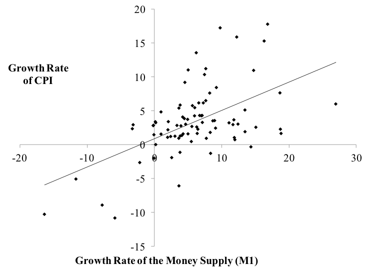
Figure 1. Annual Growth Rate of CPI and of the Money Supply
Sources: BLS, Federal Reserve
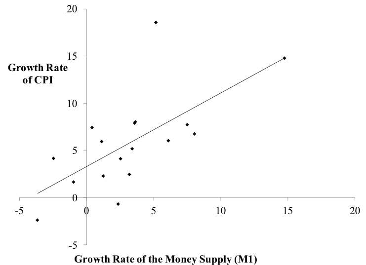
Figure 2. Five-year growth rate of CPI and of the money supply
Sources: BLS, Federal Reserve
Income distribution and inflation
Another theory of the price level starts with an identity grounded in macroeconomic accounting:
PQ ≡ W + U
This is the income approach to GDP. It says that nominal GDP (PQ) is the sum of all incomes. For simplicity, there are only two incomes: wage bill (W) and gross profit (U). All of them are measured before tax. Divide by Q on each side:
P ≡ W/Q + U/Q
W is equal to the product of the average nominal wage rate (w) and the number of hours of labor (L): W = wL (for example, if w is $5 per hour and L is equal to 10 hours, then W is equal to $50). Thus:
P ≡ wL/Q + U/Q
Q/L is the quantity of output per labor hour, the average productivity of labor (APL):
P ≡ w/APL + U/Q
w/APL is the unit cost of labor. U/Q is a macroeconomic mark-up over the labor cost. To get to a theory, the following assumptions are made:
- H1: the economy is usually not at full employment and Q (and economic growth) changes in function of expected aggregate demand (this is Keynes’s theory of effective demand).
- H2: w is set in a bargaining process that depends on the relative power of wage-earners (the conflict claim theory of distribution underlies this hypothesis)
- H3: U, the nominal level of aggregate profit, depends on aggregate demand (Kalecki’s theory of profit underlies this hypothesis, see below)
- H4: APL moves in function of the needs of the economy and the state of the economy, it is procyclical to the state of aggregate demand for goods and services. In general, in periods of labor-time scarcity gAPL goes up and, during an economic slowdown, gAPL goes down before employees are laid off.
Thus:
P = w/APL + U/Q
The price level changes with changes in the unit cost of labor and the size of the macroeconomic mark up. In terms of rates of growth:
gp ≈ (gw – gAPL)sW + (gU – gQ)sU
With sW and sU the shares of wages and profit in national income (sW + sU = 1). Thus, inflation has two sources:
- Cost-push inflation: the growth rate of the unit labor cost of labor (gw – gAPL) depends on how fast nominal wage grows on average relative to the growth rate of the average productivity of labor. The correlation between the unit cost of labor and inflation is very strong both in the “short-run” (0.82 for yearly growth rates) and “long-run” (0.93 for five-year growth rates) (Figure 3).
- Demand-pull inflation: U follows Kalecki’s equation of profit which states that the level of profit in the economy is a function of aggregate demand. Thus, the term, gU – gQ represents the pressures of aggregate demand on the economy; it is an output gap. If gU (the growth of aggregate demand) goes up and gQ (the growth of aggregate supply) is unchanged, then gP rises given everything else. However, to assume that gQ is constant is not acceptable unless the economy is at full employment. Usually, a positive shock on aggregate demand growth leads to a positive increase in aggregate supply growth because the rate of utilization of productive capacities is below one even in “the long run.”
Note that the money supply is absent from this equation. The money supply does not directly affect output prices. Spending may impact inflation but it depends on the state of the economy.
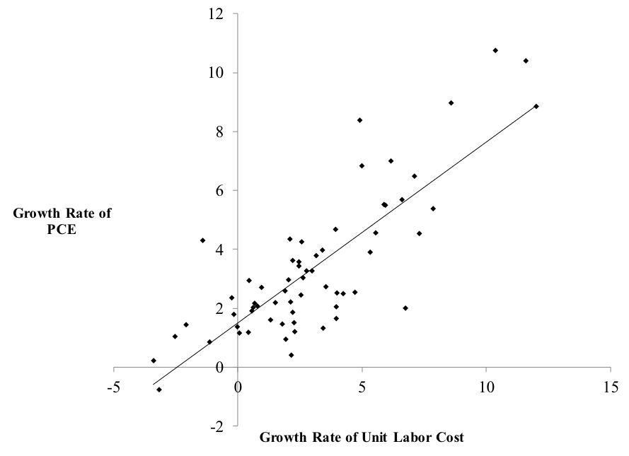
Figure 3. Annual Growth Rate of Unit Cost of Labor and Growth Rate of PCE
Source: BEA, Federal Reserve
Note that the growth rate of wage is by itself not as relevant. It is its relation to the growth rate of the average productivity of labor that matters. Time-series data provides another insight into the role of the unit cost of labor (Figure 4). From the mid 1960s to the early 1980s, unit cost of labor was a main source of high inflation. Nominal wage growth outpaced productivity growth, both grew on average. The former was in the 5-10% range whereas the latter was mostly in the 0-5% range. In the late 1960s, workers were able to outpace productivity growth because of their strength in wage bargaining due to low unemployment and strong unions. The 1970s oil shocks boosted inflation and workers tried to maintain their real wage (they failed) by demanding an increase in nominal wages. This further reinforced inflation because productivity could not keep up with wage demands. The internationalization of labor and the decline in the power of unions have tamed the ability of wages to outpace productivity even in periods of long economic growth.
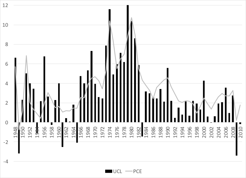
Figure 4. Unit cost of labor growth rate and inflation, Percent
Source: BEA, BLS
When combined with the explanation of monetary creation presented in Post 10, this theory of inflation provides an explanation of the correlation between price and money supply that involves a reversed causality compared to the QTM. Higher costs of production and higher demand pressures push up the price of goods and services, which increases the size of the bank advances that economic units request: higher P (gP) leads to higher M (gM).
A broader point is that the growth of the money supply is not by itself inflationary because money supply grows with the needs of the economic system, economic units are not suddenly allocated bags of money supply with which they do not know what to do:
- Firms request bank credit to start production (pay workers, buy raw material) and repay their bank debts (which destroys money supply) once production is sold: money supply moves in part with the need of the productive system
- Federal government spending (that injects money supply) and taxing (that destroys money supply) move automatically in a countercyclical fashion to tame inflationary pressures (“automatic stabilizers”): during an expansion (a recession), the growth rate of government spending falls (rises) and the growth rate of taxes rise (falls). In the US, most of the automatic stabilizer effect comes from wild fluctuations in the growth rate of taxes (in a recession economic units have less income so they are taxed less) (Figure 5).
So the money supply is not something that falls from the sky, its injection and destruction in relation to the production process must be explained and the debts incurred by monetary creation must be included in the analysis. If the economy is growing, money supply grows, if economic units do not want to hold monetary instruments they may just use them accelerate the repayment of their bank debts.
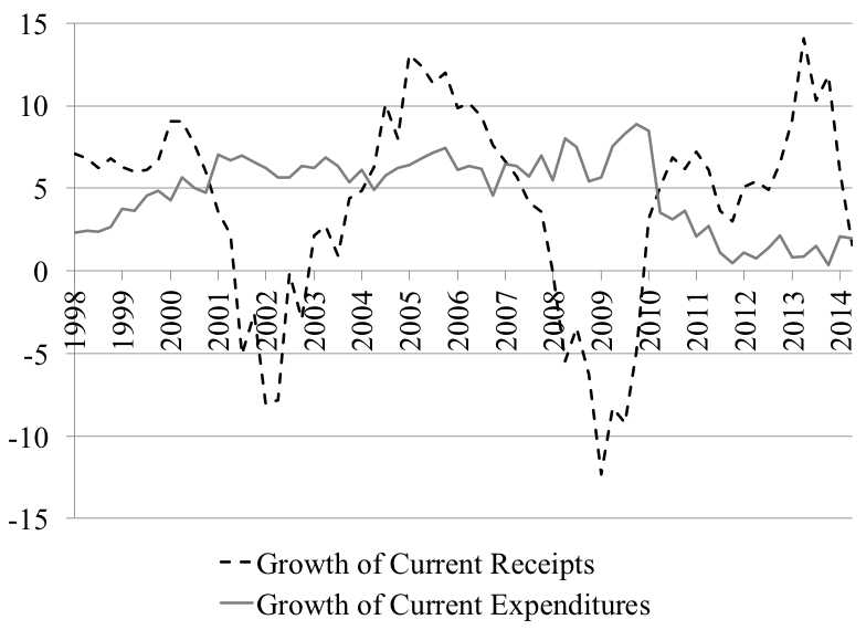
Figure 5. Automatic Stabilizers.
Source: BEA.
In terms of policy, the theory means that inflation is managed best by buffer-stock policies and income policies, or a combination of both such as a job-guarantee program. Monetary policy does not have much direct impact on inflation, and an increase in interest rates can contribute to inflation through the cost and demand impacts of higher interest rates (see below). The role of a central bank is to preserve financial stability through the provision of a stable low cost refinancing source and through regulation.
To go further: Kalecki equation of profit, interest rate and inflation
For readers who want to know more, this section develops a few points. The income-approach to GDP can be developed further to account for rentiers’ income, which, to simplify, only comes from the distribution of profit. Gross profit is the sum of net profit, non-wage income distribution, and taxes on profit:
PQ ≡ W + U ≡ W + Z + UnD + TU Þ P ≡ w/APL + Z/Q + UnD/Q + TU/Q
With, U gross profit of firms, UnD the disposable net profit of firms (i.e. profit after accounting for business income tax, distribution, and subsidies), W employees’ compensations, Z the gross non-wage incomes paid by firms (dividends, interests, rental income), and TU business income tax (tax on profit). For small values of gQ and gAPL we have:
gP ≈ (gw – gAPL)sW + (gZ – gQ)sZ + (gUnD – gQ)sUnD + (gTu – gQ)sTu
The assumptions are that gw results from a bargaining process between employees and firms. gZ depends on monetary policy and the state of liquidity preference (Z depends on the level and structure of interest rates). gAPL is procyclical to the state of the economy. gQ is determined by expectations of monetary profits (Keynes’s effective demand). As shown below, gUnD is determined by the Kalecki equation of monetary profit. Finally, the growth of profit taxes depends on the tax structure and economic activity. For the sake of the argument, one can assume that national income shares are constant and sum to one (sW + sZ + sUnD + sTu = 1).
Inflation can go up and down as gUnD, gw, gZ and gTu go up and down, but their effects will be mitigated by changes in productivity growth and output growth. Only when the latter two are fixed or sluggish relative to the former four can inflation permanently take place; this is a state of “true inflation” to take Keynes’s terminology. One economic condition during which this can occur is full employment, but this is not the only one. Prices may go up quickly because of, for example, uncontrolled wage-price spiral induced by high expectation of inflation, competition between unions for relative wage improvements, or a rise in costs not controlled by residents (e.g., oil shock). Rising interest rates also can promote inflation by raising costs of production (Post 5 noted that FOMC members are aware of this inflationary channel).
This explanation of inflation does not discard the possibility of a monetary source of inflation, but it requires that several conditions be met because the relation between money supply and inflation is highly indirect. First, if funds are injected via portfolio transactions (swapping of non-monetary assets for monetary assets), output-price inflation may occur only if desired stocks of monetary assets are fulfilled. If receivers of monetary assets decide to spend their excess funds to buy existing goods and services—they could also buy financial assets, which would lower interest rates, and/or repay their debts—and if the economy is in a sluggish state.
Second, if funds are injected in the private domestic sector via income transactions (e.g. wage payment), inflation will occur only if the economy is slow to respond (so that UnD/Q increases). The Kalecki equation of profit expresses this more formally. National accounting identities tell us that:
W + Z + UnD + TU ≡ C + I + G + NX
With C the consumption level, I the level of investment, G the level of government spending, and NX net exports. Accounting for net tax payments induced by taxes and transfer payments in all sectors one gets:
WD + ZD + UnD ≡ C + I + DEF + NX
With the subscript D indicating disposable income (i.e. after tax and transfer payments), and DEF the government budget deficit (including transfer payments). Subtracting WD + ZD from each side and defining CU as the consumption out of disposable net profit one has:
UnD ≡ CU – SH + I + DEF + NX
With SH (= SW + SZ = (WD – CW) + (ZD – CZ)) the saving level of wage earners and rentiers. Kalecki argues UnD is not under the control of firms, whereas variables on the right side (expenditures) depend on discretionary choices, so the causality runs from spending to profit. Thus:
gUnD = (gCusCu – gShsSh + gIsI + gGsG – gTsT + gXsX – gJsJ)/sTu
Where si is the share of variable i in national income (or GDP) which is assumed to be constant. As the economy gets to full employment, any type of spending (public or private, consumption or investment) will tend to be inflationary. Higher interest rates can contribute to demand-pull inflation if the growth of consumption by rentiers increases too fast as a result of higher interest income. The inflationary tendencies can be mitigated by the growth rate of tax, the growth rate of production, the growth rate of the average productivity of labor and the growth rate of saving.
[Revised 8/6/2016]
To go further: Kalecki equation of profit, interest rate and inflation やや専門的:カレツキーの利潤方程式、金利とインフレーション もうちょっと細かく知りたいという読者のため、ここでは2・3の論点に関わる付論をつける。GDPへの所得アプローチはさらに不労所得の説明に拡張することができる。これは単純に言えば、利潤の分配の所得である。総利潤は、純利潤、非労働所得分配、および利潤に対する租税の総合計である。 PQ ≡ W + U ≡ W + Z + UnD + TU Þ P ≡ w/APL + Z/Q + UnD/Q + TU/Q Uは企業の総利益は、UnD は企業の可処分利益(利潤から法人税、配当、補助金を差引したもと)、Wは従業員への報酬、Zは企業によって支払われる非賃金所得(配当、金利、賃貸料)、およびTU は法人税(利潤に対する課税)の合計となる。 小文字gQ と gAPL で書くと、 gP ≈ (gw– gAPL)sW + (gZ – gQ)sZ + (gUnD – gQ)sUnD + (gTu – gQ)sTu 仮定上、gw は従業員と企業の間の交渉プロセスの結果である。gZ は貨幣政策及び流動性選好に依存して決まる(Zは金利の水準と構造に依存する)。gAPLは経済状況のサイクルと並行している。gQ は期待貨幣利潤により決まる(ケインズの有効需要)。下記に示す通り、gUnDは貨幣利潤に関するカレツキー方程式によって決まる。最後に、法人税の成長は租税構造と経済活動水準に依存して決まる。便宜上、国民所得のシェアは変化しないものとし、それらの合計は1となる (sW + sZ + sUnD + sTu = 1) 。 インフレーションはgUnD, gw, gZ and gTu の上昇下降にあわせて、高くなり低くなる。しかしその影響は生産性及び生産額の成長率(gAPLおよびgQ)が変化することで拡大される。後の2項目が変化しないか前の4項目に比べて縮小しているとき、インフレーションは長期的に生じうる。これが、ケインズの語法で行けば「真正インフレーション」の状態ということになる。こうしたことが生じうる経済的条件の一つが完全雇用であるが、しかしそれだけではない。物価が急激に上昇しうる原因は、たとえばきわめて高いインフレ期待や、相対的な賃金改善を求める労働組合間の競争、あるいは国内居住者によってはコントロール不可能な製造コストの上昇(たとえばオイルショック)などにより、コントロール不可能な賃金―物価スパイラルが発生する、といったことが挙げられる。利子率の上昇もまた、製造原価を引き上げることでインフレーションを促進することがあり得る(ブログの第5回目で記したが、FOMCメンバーはこうしたインフレーションの経路を心配していた)。 この説明でも貨幣がインフレの発生源になる可能性を無視しているわけではない。しかし貨幣がインフレの原因になるにはいくつかの条件が必要となる。というのはマネー・サプライとインフレーションの関係はかなり間接的だからである。第一に、もし資金がポートフォーリオ取引(非貨幣性資産を貨幣資産と交換する)によって注入されるのであれば、生産価格インフレが起こるのは望ましい貨幣性資産ストックが満たされた後になる。貨幣性資産を受け取った人が超過資金を使って中古資産――あるいは金融資産(金利は低くなるだろうが)を買ったり、債務を償還するなど――を購入したり、あるいは経済が縮小していれば、やはりインフレは起こらないかもしれない。 第二に、資金が所得取引(つまり賃金支払い)を通じて国内民間部門へ注入されたとしても、インフレーションが起こるのは経済がすぐには反応しない(それゆえ UnD/Q が上昇)する場合だけである。カレツキーの利潤方程式はこれをより形式的に表現している。国民会計方程式によるなら、
W + Z + UnD + TU ≡ C + I + G + NX Cは消費水準、Iは投資水準、Gは政府支出水準、NXは純輸出である。すべての分野における租税から移転支出を差引することで純納税額が計算されるので WD + ZD + UnD ≡ C + I + DEF + NX 添え字Dは可処分所得(つまり税引後)を意味し、DEFは政府の赤字財政(移転支払を含む)を意味している。WD + ZD を両辺から差引し、可処分純利潤からの消費をCU と定義すると、
UnD SH (= SW + SZ = (WD ≡ CU– SH + I + DEF + NX – CW) + (ZD – CZ))は賃金稼得者および不労所得者からの貯蓄水準である。カレツキーによれば、UnD は企業のコントロールできるものではなく、また右辺の変数(支出)は任意の選択に依存しているのだから、因果関係は支出から利潤へと向かう。 かくして、
gUnD = (gCu sCu– gShsSh + gIsI + gGsG – gTsT + gXsX – gJsJ)/sTu ここで、si は国民所得(またはGDP)に占める変数iのシェアであり、一定と仮定されている。経済が完全雇用状態になれば、どんなタイプの支出でも(公共でも民間でも、消費でも投資でも)インフレ的になるだろう。金利の上昇は、金利所得上昇の結果として急速になりすぎれば金利所得者の消費の伸びが金利所得上昇の結果として急速になれば、ディマンド・プル・インフレーションを刺激しうる。インフレーション傾向は租税の伸び、生産の成長率、労働の平均生産性の伸び率、所得の伸び率によって、変化しうるのである。 [Revised 8/6/2016]
Primer: The Kalecki Profit Equation (Part I)

The Kalecki profit equation -- named after the economist Michal Kalecki -- describes how aggregated profits are determined by national accounting identities. (Note that Jerome Levy came up with a similar approach earlier; the equation is sometimes referred to as the Kalecki-Levy profit equation.) The results are perhaps not obvious if we look at profits from a bottom up perspective. From the perspective of business cycle analysis, the key point to note is that net investment is a source of profits. Meanwhile, since firms invest in order to grow profits, we get a self-reinforcing feedback loop. From a policy perspective, we see that governmental deficits also add to profits, which implies that increasing deficits add to profits in a recession, helping put a floor under activity.
Given the length of this discussion, it will be broken into a multi-part article. (Link to part 2.) This first article will discuss the role of savings and the distribution of income on profits. My objective is to explain the practical importance of the profit equation, and I make a number of assertions about business cycle behaviour to do so. Other articles will expand upon this analysis, and provide a stronger justification of these assertions. I also want to add a disclaimer that I am not particularly concerned about the details of national accounting; I am writing about a simplified accounting system that would reflect the outcomes of economic models. There may be some details around various definitions that I am glossing over.
If we wanted to apply the profit equation to real world national accounts data, the final equation contains a great number of terms. This complexity distracts from the basic principles of the equation. Instead, this treatment will start off with the equation for very simple model economies, and then add terms as we add complexity to the models. The usefulness of the Kalecki profit equation is for understanding the model dynamics that transfer to real world behaviour, rather than playing with national accounts identities. We can build up the equation term-by-term, and so we can have an intuition of the role of each term.
This treatment is largely based on the one found in Section 5.3.6 of Marc Lavoie's Post-Keynesian Economics: New Foundations (link to review). I would also note the historical discussion found in "Profits: The Views of Jerome Levy and Michal Kalecki [http://www.levyinstitute.org/pubs/wp309.pdf]" by S. Jay Levy; Levy's tended to be more focused on the details of the national accounts.
Given my aversion to the theoreteical concept of "money," I use "cash" in discussion. Cash can refer to any instruments that are used exchange, which may or may not be formal monetary aggregates (although all the instruments in monetary aggregates are undoubtedly cash).
Model 1: Simplest Two-Sector Model
We will start with the simplest case: an economic model with just two sectors (the business sector and workers), and no investment. Furthermore, we will assume that the business sector does not pay dividends. In order to eliminate investment, we will assume that the business either provides services or highly perishable goods; there are no inventories. We will refer to this is model #1, and it has an associated profit equation.
We will treat the business sector as if it were a single employer. If there are multiple employers, we might see that some are profitable and others run at a loss; what we are interested in is aggregate profit, so that distribution does not matter.
The business sector's profits are equal to revenue minus expenses.
- Revenue equals purchases from households.
- Expenses are equal to wages paid to workers.
We can immediately see that if households spend 100% of wages (and have no other source of spending), revenue equals expenses and profits are equal to zero. There is a circular flow of cash out of the firm to workers which then returns as revenue, and no cash drops out of the loop. However, if workers save some of their income, revenue will be less than expenses; cash has dropped out of the loop. This gives us a version of the profit equation with just one term:
(Model 1 Profits) = - (Household savings).
Even this simplest version of the profit equation has a couple interesting theoretical properties.
The first thing to note that since household savings subtract from profits, rising savings "all else equal" has a negative cyclical effect. Variants of this concept show up throughout discussions of simple monetary models; for example, the desire to hoard money could allegedly lead to a recession. However, there does not seem to be any evidence of such an effect in market economic analysis. From my perspective, the emphasis on household savings as a cyclical factor by academic economists caused me to view their work as being unrealistic. The problem is the overly simplified near-barter economies academics use to illustrate their models -- the issue is not changes in what households view as "saving," rather the willingness to incur debt.
If the household sector borrows in aggregate during the accounting period, it could consume more than it earns from wages. That is, if household saving is negative, profits are positive.
Within this two sector model, there are two avenues to allow this borrowing.
- The business sector can lend to households; for example, by offering financing on purchases. The business sector could end up with an unchanged cash balance, but it will gain financial assets -- the debt-like claims emitted by household sector.
- Individual households can lend to other households. However, this can only be sustained for as long as lending households hold cash instruments.*
Household consumption patterns appear to be fairly stable across the cycle (during the expansion, at least). However, the willingness to incur debts is more cyclical, particularly with respects to housing and car purchases.** We need to drop the parables about Farmer Bob buying apples from Farmer Alicia, or Bob's desire to hold gold coins, rather the issue is whether their kids Cynthia and Doug are buying a condo in the big city.
The next thing to note is that one could view the equation as implying that household frugality is a negative. This is in stark contrast to the conventional story that we need to increase household savings to boost growth. ("Farmer Bob needs to hold back some of his corn to plant next year!") This model stacks the deck against frugality by assuming that investment is zero; I will return to this when investment is added into the model.
Model 2: Dividends
The next addition to the model is to add dividends into the mix. Neoclassical models have a hard time with dividends, for reasons that will be discussed below. However, the inclusion of dividends into the equation has some major theoretical and political economy effects.
A dividend is a payment by a firm to its owners, and dividend income is normally the objective for capitalist firms. The normal assumption is that dividends are paid out of profits (current or historical) -- although the private equity industry has mucked that belief up.
Dividends and wages are the two main cash flows from the business sector to the household sector in economic models. (In the real world, some individuals either are self-employed or part of private partnerships that end up being lumped in the household sector in the national accounts. As a result, real world data could see more types of interactions than the tidy world of economic models.) Although the cash flows may be fungible, they have very different implications for profits: dividends are not an expense.
If we assume that the household sector has zero savings, all business cash outflows return in revenue. So if 20% of outflows are dividends, only 80% of outflows are wages. This means that profits (revenues minus expenses) are 20% of revenue -- or equal to the dividend payments. However, the household savings is generally non-zero, and we end up with the profit equation #2, with an added term:
(Model 2 Profits) = - (Household savings) + (Dividend payments).
(In other words, we added another term to the equation.)
One typical way to present Kalecki's model is to add some behavioural information that acts to constrain outcomes. The assumption is that workers and capitalists are distinct sets of households, and that workers spend 100% of their wages (and do not dis-save). This has the implication that that household sector saving is exactly equal to the savings of the households that receive dividends.
This implies a different profit equation:
(Kalecki Assumption Profits) = (Dividend payments) - (capitalist savings),
which by definition of savings implies:
(Kalecki Assumption Profits) = (Capitalist consumption).
This explains Kaldor's aphorism***:
Capitalists earn what they spend, and workers spend what they earn.
Once again, this version of the equation only holds in models with the constraint that workers' aggregate savings are exactly equal to zero; this will not be true in real world data (except as a statistical fluke). Furthermore, since workers and salary owners can also own equities (courtesy of the move to self-directed retirement schemes), we have a blurring in the distinction between "workers" and "capitalists." Nevertheless, it does seem safe to argue that dividend income is largely received by the upper income quantiles, and those quantiles have a greater propensity to save. Therefore, the behavioural constraint might be a reasonable approximation of reality.
The addition of the dividend term to the profit equation has limited real world significance in terms of cyclical analysis. Over short spans of time, dividends are stable, and so this term is not too significant a source of volatility when compared to the other terms to be added. Over multi-decade periods, the changes in dividend policy would presumably show up in secular profit trends, and so assertions about the long-term would need to take dividend changes into account. However, the addition of dividends to the profit equation is very important from a theoretical perspective, as well as for political economy.
(The current popularity of stock buybacks might muddy the theoretical waters. In a stock buyback, the business sector outflows are in exchange for financial assets, and the seller will not count the sales proceeds as normal income. At most, there will be capital gains. Trying to analyse this properly would require something like a stock-flow consistent model that takes into account equity market valuations and capital gains. Those models are complex, and raise a great number of thorny questions. I may return to this question, but I do not see an obvious answer as to the macro effects of a switch from dividends to stock buybacks.)
The theoretical problem with dividends being a source of profits is that is creates a self-reinforcing feedback loop between profits and dividends, as greater profits allows for greater dividends. For simpler models like stock-flow consistent models, this is not a particular issue. However, if one believes that model outcomes are in some sense the result of optimising behaviour, this creates difficulty. If the business sector (or capitalists) were truly aiming for optimal outcomes, the solution would likely be pathological, with extremely high dividends that are not saved. Neoclassical models avoid these problems by avoiding actual optimisations, instead sectors follow heuristics that are sub-optimal relative to choices that are implied by taking into account the full macro model. (See this article for a longer explanation of that assertion.) This accords with my previous experience in applied mathematics: for practical problems, optimisations almost always result in pathological outcomes.
Even if we accept that economic outcomes are not in any sense optimal, there are important implications of the role of dividends. The implication is that the level of profits in an economic system are essentially arbitrary; for any level of output, we can split the output between workers and capital and have a system that respects cash flow constraints (accounting identities). An economic model needs to pin down the distribution of income using some assumptions about behaviour in order to have a single solution.
Neoclassical models hide distributional questions under the carpet by assuming that workers and capital receive their just desserts: marginal contributions determine the levels of wages and profits, and hence the income shares. As a result, it is possible to ignore the politics of income distribution. By contrast, the post-Keynesian tradition explicitly notes the arbitrary nature of income distributions. To be fair, "mainstream" economists are now more willing to discuss the effects of income distribution (at least the leftward end of the mainstream).
From a short-term perspective, distributional questions are a second order effect. I have seen arguments to the effect that the structural sluggishness of recent decades is due to a lower wage share of national income, but I am agnostic on the validity of that view. Investment trends are much more important for profit determination, as I discuss next.
Model 3: Investment
I will conclude this part of the article with the addition of investment, which is arguably the most important cyclical component during an expansion. For those who are new to economics, one needs to keep in mind that the definition of "investment" in economics does not match the way the word is often commonly used. For example, people will often use "investing in the stock market" as a way of describing the purchase of shares; this does not fit the definition used in economics. Instead, "investment" here refers to spending by firms that creates non-financial assets that presumably will generate future profits. The trick is that this can either be fixed investment, or investment in inventories. The issues around inventory investment will be discussed later.
(The usual convention in the national accounts is that investment is largely an activity of the business sector; household spending is usually classified as consumption. This is an artefact of the nature of the way that national accounts are measured. For example, national statisticians cannot tell whether my purchase of a computer is to support consulting activities -- an investment -- or to play the latest video games -- which is a form of consumption. The discussion here follows the convention that only the business sector invests.)
Investment is another cash outflow by businesses that is not an expense. As a result, circular flows result in revenue that is not matched by a wage expense -- profits.
The Model 3 equation now reads:
(Model 3 Profits) = (Net Investment) - (Household savings) + (Dividend payments).
The transactions for investment are more complicated than the previous models. We can imagine three basic channels for investment in this simplified framework. (If we add more sectors, there are more possibilities.)
- The firm pays workers $100 to create a capital good. The $100 payment is not treated as an expense, it is instead "capitalised." From the workers' perspective, it does not make a difference whether the $100 is expensed or not; it is a household income-producing cash flow that can be spent. The household cash flow then recirculates through the system as before. Profits are higher since we are now no longer deducting some of the cash flows from revenue.
- The firm pays workers $100 to produce products that are not sold. The unsold products will end up in inventory. The inventory will be held on the balance sheet at the production cost (which is equal to to wage payments need to produce the goods). The hope is that the goods in inventory will be sold in a future accounting period, and the profits on the sale are equal to the sales price less the cost of the goods as valued in inventory. (Under most circumstances firms cannot mark the value of inventories as equal to their final selling price, as firms could generate "profits" by just producing goods that cannot be sold and dumping them into inventory.) This then leads to another observation -- selling the goods out of inventory represents disinvestment (negative investment), and this amount would be subtracted from gross investment in the next accounting period to get net investment. (Note that the profit equation specifies net investment, not gross investment.)
- Firm A purchases a capital good for $100 from Firm B. Firm B held the good in inventory, with a value of $80. The $100 cash outflow for Firm A is not an expense; and so the transaction is profit neutral. For Firm B, the profit on the transaction is equal to the selling price ($100) less the cost of goods sold ($80) -- which implies a profit of $20. The net investment for the aggregate business sector is also $20. Firm A has a new fixed investment of $100, while Firm B has an inventory disinvestment of $80. It is easy to see that cash flows can get quite complicated once we allow for intra-sector cash flows (e.g., business to business flows). For example, an investment project could have a mixture of purchased inputs as well as worker pay. The key is that investment creates outflows that are not matched to an expense.
Depreciation adds another wrinkle to the concept of net investment. Most capital goods have a finite lifespan, and their value is written down over time. The decrease in asset value is known as depreciation, and it shows up as an expense (the cost of capital). Depreciation is subtracted from other investment in order to get net investment. That is,
Net Investment = (Gross fixed investment) - (Depreciation) + (New goods added to inventory) - (Value of goods sold from inventory).
If we had a static economy with fixed nominal prices, depreciation expense would converge to equal gross investment. For example, assume that all capital goods depreciate by 10% of their initial value every year for 10 years. If firms invest $100 per year, that would create an expense of $10 per year for 10 years. After doing this for 10 years, the level of depreciation expenses would equal the new investment. However, the usual condition for modern economies (outside Japan) is that prices and volumes of investment are rising over time, so the new investment is larger than the depreciation of earlier investments (which have a lower nominal value).
The net investment component of the profit equation is much more important from a cyclical perspective than household saving and dividends. The reason is that investment is pro-cyclical: firms invest if they expect higher future demand -- and profits. Since investment itself generates profits, expectations of higher profits can be viewed as self-fulfilling. This means that expansion is the natural state for capitalism; the problem is that other factors can derail profits and investment, and then the self-reinforcing feedback depresses activity.
I would summarise the post-Keynesian view of how firms operate during an expansion as follows. (I will fill in references in later.) It is a mistake to believe that firms attempt to solve some optimisation problem in order to plan their activities; they are missing too much useful information to fill in the optimisation parameters. Instead, they need to use rules of thumb (heuristics), such as extrapolating past growth trends. Obviously, they do a great deal of analysis of their market, but there is an obvious great amount of uncertainty about the direction of the overall economy. They will then come up with some baseline forecast of demand for their products.
- They will plan production to meet demand, and to grow their inventories in line with sales. That is, they typically want to keep the ratio of inventory to sales at some target ratio, such as holding one month's sales in inventory. (Since inventory is a stock and sales are a flow, the ratio has units of time.)
- They will launch fixed investments if they believe that they need to add capacity to meet projected demand.
The implication is that if firms are projecting demand growth over their planning horizon, they will generally plan on both increasing inventories as well as increasing fixed investment.
The future does not always meet past projections. Two competing firms may have ramped up capacity beyond the demand for their products, and so sales end up below their projections. If they are producing goods that are held in inventory, they will end up with a higher inventory-to-sales ratio than desired. By itself, the higher inventory levels do not cause a loss. However, the unplanned inventory build represents a hit to cash flow -- they paid cash to produce the inventory. Their balance sheet weightings shift from cash to inventories -- and they need cash to meet expenses and repay debts. The inventory build has to be reversed -- which implies a reduction in investment.
This means that "investment" is not an unalloyed positive, as it is sometimes portrayed in economic parables. One very often encounters stories about Robinson Crusoe economies, or economies that consist of barter among various proprietors (fisherman, shoemakers, etc.). In such an exchange economy, investment is represented as frugally abstaining from consuming output to add to productive capacity. However, in a monetary economy, "investment" may just be the piling up of unsold goods at firms -- and those firms will go bankrupt if that inventory build is not reversed. This explains why "Keynesian" economists often emphasise the role of demand within the economy.
Concluding Remarks
The discussion of the Kalecki Profit equation will conclude with the addition of two extra terms, which take into account the government and external sectors.
Link to the second part.
Footnotes:
* These sorts of complicated intra-sector transactions can break overly simplistic analysis that wants to develop mechanistic models of cash flows in the economy. As a result of things like intra-sector borrowing, measured gross debt levels can move around without resulting in changes in measured GDP. Conversely, if one assumes that debt is only issued to purchase goods and services, one can incorrectly believe that there is an iron law relating debt changes to GDP changes.
** The purchase of an existing house does not itself add to GDP, whereas it will inflate household debt (in the typical case where the buyer will end up with a larger mortgage than the seller). This makes sense, as we do not consider the proceeds of a house sale to be income. That said, there are fairly large income effects in a typical housing transaction. Things like realtor fees, mortgage insurance, legal fees, welcome tax, and moving expenses represent income for the providers of services, and are often rolled into the mortgage. As a result, a portion of the increase in mortgage debt does directly raise GDP. This matches up with the experience of housing booms: they buoy economic activity, but the effect is smaller than the change in mortgage debt would imply.
*** N. Kaldor, "Alternative Theories of Distribution," Review of Economic Studies, 23 (2), pages 83-100. The quote itself is in page 96. I got the reference from Marc Lavoie's Post-Keynesian Economics: New Foundations. He notes that this quotation is often mis-attributed to Kalecki.
(c) Brian Romanchuk 2018
Primer: The Kalecki Profit Equation (Part II)

This article continues the discussion of the Kalecki Profit Equation (link to Part I). The Kalecki Profit Equation is an account identity (a statement that is true by definition) that determines the level of aggregate business sector profits in terms of other national accounts variables. The full equation is somewhat imposing, so the strategy employed here is to build up the equation by starting off with a simplified model economy that results in a brief equation, then adding new terms progressively. The previous article noted that investment creates a pro-cyclical self-reinforcing loop between it and profits. This article discusses two factors that normally act to moderate the business cycle: the fiscal deficit, and the external sector.
As in the previous article, the treatment here is aimed at the simplified economic model accounting, and not the full details of the national accounts. If one wanted to apply the accounting identity to real world national accounts, there are a great many smaller terms that would need to be added in in order to get the full accounting identity.
Model 4: Government Fiscal Policy
The previous article started off with a simple two sector economic model, with the two sectors being the business sector and households. The last model considered was Model 3, and had an associated profit equation:
(Model 3 Profits) = (Net Investment) - (Household savings) + (Dividend payments).
We will now add a third sector: the general government sector. We will label this Model 4.
(Model 4 Profits) = (Net Investment) - (Household savings) + (Dividend payments) + (Government Fiscal Deficit).
The addition of the government sector added the final term to the equation -- the fiscal deficit. This is a fairly conventional phrasing, but it must be kept in mind that the fiscal deficit is the negative of the fiscal balance, so we need to flip signs if we want to use the fiscal balance as the variable. The usual condition for governments is to run deficits, so it is more familiar to express the equation using it.
The reason why a fiscal deficit creates profits is that the government is now injecting cash into the circular flows in the economy. If the government mails a senior a $100 transfer payment, and said senior immediately runs out and spends it, that represents $100 in business sector revenue that is not matched to any wage expenses.
(I am following the convention of economic models, and treating government spending as consumption. If governments capitalised some investment expenditures, those expenditures might not be considered part of the fiscal deficit, and they would need to be added into the profit equation.)
For profits, the full fiscal balance matters, not just the primary balance (the balance excluding interest payments). Mainstream economic analysis often likes to focus on the primary balance, but this glosses over the reality that interest payments by the government are an income source to the non-governmental sector.
The presence of the fiscal deficit in the profit equation is an important part of the counter-cyclical nature of fiscal policy. Mainstream economic models attempt to gloss over the the importance of profits on the basis that competition allegedly causes profits to wither away. However, in a recession, deficits naturally grow -- the tax take falls, while welfare state spending (such as unemployment insurance) automatically increases. Furthermore, even fiscal conservatives tend to panic in a downturn, adding active stimulus measures to the mix. The rising contribution of the fiscal deficit will counter-act the drop in investment, putting a floor under profits (and animal spirits) in the private sector.
During an expansion, fiscal deficits tend to contract (or least grow less than GDP in nominal terms). This acts as an increasing drag on profits, counter-acting the pro-cyclical impetus from investment.
In summary, a focus on the interaction between the fiscal deficit and profits gives a much greater weight on fiscal policy than an approach based on appealing to the so-called inter-temporal governmental budget constraint would suggest.
Model 5: The External Sector
The final addition to the profit equation is to bring in the external sector (imports and exports). If a country has net imports of goods, it implies that net cash flows are heading to foreign entities -- implying a loss in the circular flow of income.
The addition of the external sector adds a new wrinkle -- the profits that we are discussing here are domestic profits, which is not the same thing as national profits. A local firm may have profits in its foreign subsidiaries, but those will not show up in the domestic national accounts. A stock market investor is interested in the total profits of firms, and not just domestic profits, so the distinction needs to be kept in mind.
(Model 5 Profits) = (Net Investment) - (Household savings) + (Dividend payments) + (Government Fiscal Deficit) - (Net Imports).
The breakage in cash flows is straightforward. If a worker spends $100 on imported goods out of wage income, the source of the wages was an expense to the domestic business sector, while the domestic sector gains no revenue.
This raises a different perspective on the question of protectionism. From the perspective of optimising decisions of households, free trade is an obvious advantage, as it opens the opportunity set for consumption purposes. However, a trade deficit is a negative for domestic corporate profits.
If we assume that imports as a percentage of total domestic consumption is stable (the propensity to consume), import growth will equal the domestic growth rate. Meanwhile, exports would tend to grow at the growth rate of our export markets. The implication is that if our domestic growth rate is greater than elsewhere, the trade balance will tend to fall. For the "Anglo" countries (such as the United States) in recent decades, trade deficits will tend to rise during an expansion. As a result, the external sector will tend to act in a stabilising fashion for profits. This will be less true for countries following an export-led growth dynamic, as the persistent trade surplus will tend to move in tandem with the global business cycle.
Concluding Remarks
We have slowly built up the Kalecki Profit equation to a fairly general form. We would need to adapt it to take into accounts various technicalities in the national accounts if we wanted to apply it to real world data. I am unconvinced about the value of such an exercise, since it is unlikely that we could forecast each of the components of the full equation. Meanwhile, if we are not interested in forecasting, we can just read off profits from the national accounts, rather than calculating them with an accounting identity. Instead, the value of the accounting identity is for the analysis of models, and getting a high level understanding of the nature of the dynamics.
For example, one notes that the wage bill does not appear in the equation. That is, rising wages are not necessarily a negative for profits -- which is not obvious if we pursue a bottom up microeconomic perspective. Rising wages would presumably allow for greater household savings (which does appear in the equation), but that is a second order effect.
However, the most important take away is the importance of investment for the business cycle. Businesses invest on the expectation of greater future profits -- and investment is a source of aggregate profits. Central banks playing around with the money supply is at most a speed bump in the way of the self-reinforcing growth dynamics of industrial capitalism.
From a policy perspective, Minsky argued that this accounting logic implies the need for a relatively large central government to tame the business cycle. Small governments (5-10% of GDP, which was relatively normal peacetime share pre-World War II) will not generate a large enough cyclical swing in the fiscal deficit to cancel out the fixed investment cycle. The absence of the automatic stabilisers allows what would be recessions turn into depressions.
(c) Brian Romanchuk 2018




8 Comments:
円安政策は貧困層にとっての生活必需品の値段を上げ
企業本体を外資に買い叩かれて終わった
江口氏は昔からMMTを馬鹿にしてきた
理解せずに
それを修正して今度は当たり前の事だと言ってきた
レイの予言の通りだ
自分の専門のDSGEからMMTを分析すればいいのに出来ないのは
DSGEが間違いだとバレるから
Yは所与ではないし均衡は前提ではない
失業率、負債率、労働分配率、
変数はこの3つでいい
江口氏は昔からMMTを馬鹿にしてきた
理解せずに
それを修正して今度は当たり前の事だと言ってきた
レイの予言の通りだ
自分の専門のDSGEからMMTを分析すればいいのに出来ないのは
DSGEが間違いだとバレるから
Yは所与ではないし均衡は前提ではない
失業率、民間負債率、労働分配率、
変数はこの3つでいい
奥本聡 (@satosiokumoto13)
2020/04/26 10:40
おー。MMT論者や財政拡大派に対して、金の亡者という藁人形があるのを初めて知りました。
MMT論者は実物との結びつきで財政拡大を言っているので、金の亡者ではないと思う。
むしろ、ETF買いを支持している人が、金の亡者的だよね。 twitter.com/yukkuri_libera…
https://twitter.com/satosiokumoto13/status/1254223774540431360?s=21
ティモワーニュhttps://love-and-theft-2014.blogspot.com/2020/09/blog-post_25.html @
Eric Tymoigne (@tymoignee)
2020/12/17 3:08
Exam question in my Modern Money Theory Class. Requires at least a one-page answer. You have one hour pic.twitter.com/maXOyJQ7Km
https://twitter.com/tymoignee/status/1339271260665073665?s=21
763 名無しさん@お腹いっぱい。[] 2022/05/03(火) 17:33:54.08 ID:z3rq+lji
と、思ったんだが、
今年1月の共通試験で、
信用創造の問題が出て、
万年筆マネーにシフトして、
https://i0.wp.com/megumino-clinic.com/wp-content/uploads/2022/01/s-keizai_205.gif?resize=620%2C876&ssl=1
一部で若干、話題になってたみたいだね。
案外、切り替わりが早い?
いつから、
学習指導要領が切り替わったんだろ?
参考ページ
https://megumino-clinic.com/2795.html
https://blog.goo.ne.jp/wankonyankoricky/e/8e8ce31546802807a238f5069e0b3751
興味深いのは、
いわゆるちゃんとした御用経済学者や、
著名な御用経済アナリストとかが、
ほとんど触れてない点か?
「共通試験 信用創造」
で検索すると記事がいろいろと出てくる。
共通試験高校政治経済の信用創造の説明が変わったことについて - 断章、特に経済的なテーマ
https://blog.goo.ne.jp/wankonyankoricky/e/8e8ce31546802807a238f5069e0b3751
2022年4月8日
断章、特に経済的なテーマ
22/01/30 08:56
レイ&ティモワーニュの'Rise and Fall of Money Manager Capitalism' では証券化・ストラクチャー化が進展した結果として、銀行は組成した融資を最後まで面倒見る必要がなくなったことが重視されているんだけれど、それ以前は融資先のビジネスが破綻すれば金利収入と貸付残金が失われるわけだから、危機に陥ったビジネスをどうするのか、低コストで再生できれば一番いいけれど、その判断をどうするのか、これが銀行ビジネスにとって重要なノウハウだったというわけで、で、証券化・ストラクチャー化はこうしたくびきから銀行を解放したんだ、それがMMC隆盛にとって極めて重要なポイントだったんだってこと。逆に言えば、こうしたくびきをそのままにした状態で証券化はまだしもストラクチャーかなんか、したくたってできない、しても結局効果はないんだよね。こういう金融商品って発行するときは購入者にいい顔できるからいいんだけれど、いざ債務者が危機に陥り、それを資金提供者が「社会的責任」とかいう理由で何とかしなきゃならない、というときには手間が増えるばっかりで、結局意味なくなっちゃうんだよね。つまり金融自由化、証券化、ストラクチャー化、、、、こうしたことを駆使して利益を上げまくろうとするなら、社会的責任なんて負った存在じゃあり続けられない。社会的責任――例えば自分の負債を通貨として発行できる――なんてことからは自由でなければ(あるいはそう周囲に信じてもらっていなければ)ならない。でも実際には保護だけは受けるけれど、責任は負わない――これが金融自由化の一面でもあったわけで、それを世間に悟られないようにするためには内生説であってはならなかった。
chocolate croissant?
cf.
https://twitter.com/tymoignee/status/1313317156004589569?s=21
https://twitter.com/tiikituukahana/status/1521705159319224321?s=21
コメントを投稿
<< Home